Clopidogrel PBPK-PD in CAD with or without diabetes (Xu 2020)

Model and source

Xu et al. (2020) built a whole-body physiologically based pharmacokinetic-pharmacodynamic (PBPK-PD) model for clopidogrel (CLOP), its intermediate 2-oxo-clopidogrel (2-oxo-CLOP) and its active thiol metabolite (CLOP-AM, the H4 isomer). The PD endpoint is inhibition of platelet aggregation (IPA). They built the model for healthy adults and then scaled it to coronary artery disease (CAD) patients with or without diabetes mellitus (DM).

mod <- readModelDb("Xu_2020_clopidogrel_pbpk")

• Citation: Xu RJ, Kong WM, An XF, Zou JJ, Liu L, Liu XD (2020). Physiologically-Based Pharmacokinetic-Pharmacodynamics Model Characterizing CYP2C19 Polymorphisms to Predict Clopidogrel Pharmacokinetics and Its Anti-Platelet Aggregation Effect Following Oral Administration to Coronary Artery Disease Patients With or Without Diabetes. Front Pharmacol 11:593982. doi:10.3389/fphar.2020.593982. Equations 1-18; physiology from Table 1; physicochemical parameters and Kt/p from Table 2; CYP kinetics from Table 3; all other values from the Methods text.
• Article: https://doi.org/10.3389/fphar.2020.593982 (open access, PMC7845657)
• Description: PBPK-PD (whole-body, perfusion-limited, Phoenix WinNonlin 8.2). Clopidogrel, 2-oxo-clopidogrel and the active thiol metabolite (CLOP-AM, H4) with inhibition of platelet aggregation (IPA) after oral clopidogrel in a 70-kg adult, with CYP2C19 phenotype (UM/EM/IM/PM), coronary artery disease (CAD) and diabetes mellitus (DM) covariates. Fourteen perfusion-limited tissue/blood compartments per analyte (lung, heart, spleen, liver, kidney, brain, adipose, muscle, skin, rest of body, stomach wall, venous and arterial blood) plus five gut-wall segments. Oral clopidogrel empties from the stomach lumen through a five-segment gut lumen; the duodenum, jejunum and ileum absorb it with P-gp efflux back to the lumen. Hepatic CYP1A2/2B6/2C19 Michaelis-Menten oxidation forms 2-oxo-clopidogrel, CYP2B6/2C9/3A4/2C19 oxidation of 2-oxo-clopidogrel forms CLOP-AM, and CES1 hydrolysis inactivates all three analytes. Unbound venous CLOP-AM irreversibly inactivates platelets in a turnover model of normalized maximal platelet aggregation M, and IPA = (1 - M) * 100. CAD lowers all blood flows to 0.9-fold and platelet responsiveness (kirre) to 0.7-fold; DM rescales CYP and CES1 activities and replaces the gastrointestinal transit rates. Deterministic typical-value model (the variances of the paper’s visual predictive check were not reported).

Structure (paper Figure 1 and Equations 1-18):

• Each of the three analytes has the same perfusion-limited body (Eq 1): lung, heart, spleen, liver, kidney, brain, adipose, muscle, skin, rest of body (ROB), stomach wall, venous and arterial blood, and five gut-wall segments. Tissue t returns blood at C_t / Kt/b, where Kt/b = Kt/p / Rbp.
• Oral clopidogrel empties from the stomach lumen (Eq 2) through five gut-lumen segments (Eq 3). The duodenum, jejunum and ileum absorb it at Ka,i and the gut wall returns unbound drug to the lumen at the P-gp efflux constant Kb,i (Eqs 4-9). The cecum and colon do not absorb.
• The liver (Eqs 11-15) receives hepatic-artery flow plus the stomach, spleen and gut-wall outflows. CYP1A2, CYP2B6 and CYP2C19 Michaelis-Menten oxidation of unbound clopidogrel forms 2-oxo-CLOP. CYP2B6, CYP2C9, CYP3A4 and CYP2C19 oxidation of 2-oxo-CLOP forms CLOP-AM. CES1 hydrolysis inactivates all three analytes. The microsomal kinetics are scaled to the whole liver by the microsomal protein content PBSF (Eq 12).
• PD (Eqs 16-17): unbound venous CLOP-AM irreversibly inactivates platelets: dM/dt = kin - kout * M - kirre * C_ven,AM * fub,AM * M, M(0) = 1, and IPA = (1 - M) * 100.
• Covariates: CYP2C19 phenotype sets the CYP2C19 Vmax of both oxidation steps (UM 1.58-fold, IM 0.5-fold, PM 0 relative to EM). CAD scales every blood flow by 0.90 (Eq 18) and kirre by 0.7. DM rescales the CYP and CES1 activities and replaces the gastrointestinal transit rates.

Population

The physiology is a 70-kg reference adult (Table 1; the listed volumes sum to 70 L). The model is a bottom-up prediction model. Its structural parameters come from in vitro kinetics (Kazui 2010 microsomal Vmax/Km, Caco-2 permeability) and the literature. The only parameter fitted to in vivo data is kirre, which was fitted to one published IPA-time profile (Zhu 2008). The comparison data are published healthy-volunteer studies (15 PK and 12 IPA reports) and studies in CAD (5 reports) and CAD + DM (5 reports) patients from East Asia, Europe and North America. Doses range from single doses of 75-900 mg to 300/75 mg and 600/150 mg loading/maintenance regimens. The paper’s visual predictive check estimated variances on Vmax,CYP2C19, CLint,CES1, Kt,i and kirre, but it did not report them, so the packaged model is typical-value only. The same information is available as rxode2::rxode(mod)$population.

Source trace

Every ini() value carries an in-file comment that points to its source.

Quantity	Value(s)	Source
Organ volumes and blood flows (healthy)	Table 1, 18 rows	Table 1 ‘Health’ columns
CAD blood-flow scaling	0.90 x every flow	Eq 18 and text (Rerych 1978); Table 1 ‘CAD’ columns
fu, Rbp, fumic (CLOP / 2-oxo / AM)	0.02 / 0.0742 / 0.0791; 0.57 / 0.68 / 0.58; 0.015 / 0.180 / -	Table 2
Kt/p for 11 tissues x 3 analytes	Table 2	Table 2 (Schmitt 2008 method)
Gastric emptying Kt,0	4.8 1/h	Methods ‘In stomach’
Transit Kt,1..5	4.2, 1.8, 2.4, 0.18, 0.06 1/h	Methods ‘In gut lumen’
fugut	0.02	Methods ‘In gut lumen’
Ka,1..3 / Kb,1..3	0.21, 0.26, 0.29 / 0.07, 0.12, 0.16 1/h	Methods, after Eqs 7-8
Microsomal Vmax, Km, enzyme content	Table 3	Table 3 (Kazui 2010)
PBSF	55,120 mg	Methods ‘In liver’
CLint,CES1 CLOP / 2-oxo / AM	276,650 / 2,200 / 529 L/h	Methods ‘In liver’
CYP2C19 UM / IM / PM activity	1.58 / 0.5 / 0 x EM	Methods ‘In liver’; Table 3 footnotes b-c
DM CYP1A2/2B6/2C9/2C19/3A4 and CES1	1.23 / 0.55 / 1.26 / 0.54 / 0.62; 1.27	Methods ‘PBPK-PD Model in CAD Patients With DM’
DM transit, stomach..colon	2.31, 2.30, 0.99, 1.32, 0.20, 0.04 1/h	same section
kout, kin, M0	0.007804 1/h, kout * M0, 1	Methods ‘PD Kinetics’
kirre (healthy) and CAD factor	47.576 mL/nmol/h; 0.7	Methods ‘PD Kinetics’; ‘CAD Without DM’
Molecular weights	321.82 / 337.82 / 355.83 g/mol	not printed; see Assumptions
Tissue, liver and gut-wall mass balances		Eqs 1, 3, 9-11, 13, 15
Lung, venous and arterial blood pools		standard closure (not printed; see Assumptions)

Two checks confirm the table values. First, the Table 1 flows close exactly: the systemic organ flows plus the stomach and gut-wall flows sum to the 5.27 L/min cardiac output. Second, the printed CES1 clearance of clopidogrel is in L/h. With the Table 3 kinetics and PBSF, the linear-range CYP intrinsic clearance is about 46,000 L/h, so CES1 is 86% of the total. The paper states “85%”.

Simulation helpers

# One deterministic typical subject per treatment. Doses go into the stomach
# lumen; observation rows carry dvid = 1 (every output is computed on every
# row). Phenotype and disease are per-subject covariate columns.
make_subject <- function(id, treatment, dose_times, dose_amts, UM = 0, IM = 0,
                         PM = 0, IHD = 0, DIAB = 0, obs_times) {
  doses <- data.frame(
    id = id, time = dose_times, evid = 1L, amt = dose_amts,
    cmt = "stomach", dvid = NA_integer_
  )
  obs <- data.frame(
    id = id, time = obs_times, evid = 0L, amt = NA_real_,
    cmt = NA_character_, dvid = 1L
  )
  out <- rbind(doses, obs)
  out <- out[order(out$time, -out$evid), ]
  out$CYP2C19_UM <- UM
  out$CYP2C19_IM <- IM
  out$CYP2C19_PM <- PM
  out$DIS_IHD <- IHD
  out$DIS_DIAB <- DIAB
  out$treatment <- treatment
  out
}

phenotype_flags <- function(ph) {
  list(UM = as.integer(ph == "UM"), IM = as.integer(ph == "IM"), PM = as.integer(ph == "PM"))
}

solve_typical <- function(events, params = NULL) {
  out <- rxode2::rxSolve(mod, events = events, params = params, keep = "treatment",
                         returnType = "data.frame")
  as.data.frame(out)
}

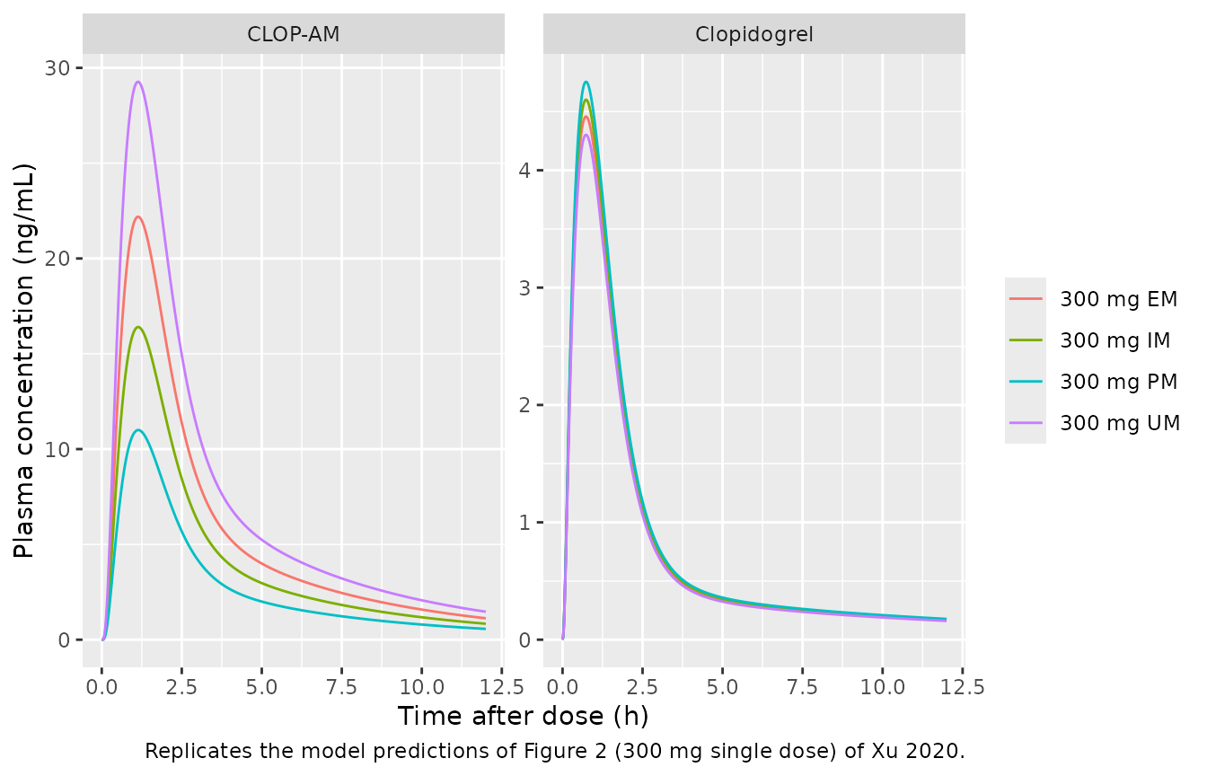
Healthy volunteers: single oral doses (Table 4, Figure 2)

single_grid <- sort(unique(c(seq(0, 6, by = 0.02), seq(6, 24, by = 0.25))))
single_design <- tidyr::expand_grid(dose = c(75, 150, 300, 600), phenotype = c("UM", "EM", "IM", "PM"))
single_events <- bind_rows(lapply(seq_len(nrow(single_design)), function(i) {
  f <- phenotype_flags(single_design$phenotype[i])
  make_subject(
    id = i, treatment = paste0(single_design$dose[i], " mg ", single_design$phenotype[i]),
    dose_times = 0, dose_amts = single_design$dose[i],
    UM = f$UM, IM = f$IM, PM = f$PM, obs_times = single_grid
  )
}))
sim_single <- solve_typical(single_events)
#> Warning: multi-subject simulation without without 'omega'

sim_single |>
  filter(grepl("^300 mg", treatment), time <= 12) |>
  select(time, treatment, Clopidogrel = Cc, `CLOP-AM` = Cc_h4) |>
  pivot_longer(-c(time, treatment), names_to = "analyte", values_to = "conc") |>
  ggplot(aes(time, conc, colour = treatment)) +
  geom_line() +
  facet_wrap(~analyte, scales = "free_y") +
  labs(
    x = "Time after dose (h)", y = "Plasma concentration (ng/mL)", colour = NULL,
    caption = "Replicates the model predictions of Figure 2 (300 mg single dose) of Xu 2020."
  )

NCA with PKNCA

The paper reports one predicted Cmax and one predicted AUC per dose and phenotype (Table 4, ‘Pre’ columns). It does not state the AUC window. Cmax does not depend on the window, so it is the primary comparison. For AUC the vignette reports AUC0-24 and the two windows that come closest to the paper’s values; see the Assumptions section.

nca_one <- function(sim, events, conc_col, analyte, start, end, partial_end) {
  conc <- sim |>
    filter(!is.na(.data[[conc_col]])) |>
    transmute(id, treatment, time, conc = .data[[conc_col]])
  dose <- events |>
    filter(evid == 1, time >= start, time < end) |>
    distinct(id, treatment, time, amt)
  conc_obj <- PKNCA::PKNCAconc(conc, conc ~ time | treatment + id,
                               concu = "ng/mL", timeu = "h")
  dose_obj <- PKNCA::PKNCAdose(dose, amt ~ time | treatment + id, doseu = "mg")
  intervals <- data.frame(
    start = c(start, start), end = c(end, partial_end),
    cmax = c(TRUE, FALSE), tmax = c(TRUE, FALSE), auclast = c(TRUE, FALSE),
    aucint.last = c(FALSE, TRUE)
  )
  res <- PKNCA::pk.nca(PKNCA::PKNCAdata(conc_obj, dose_obj, intervals = intervals))
  as.data.frame(res$result) |>
    mutate(analyte = analyte) |>
    select(analyte, treatment, PPTESTCD, PPORRES)
}

nca_single <- bind_rows(
  nca_one(sim_single, single_events, "Cc", "Clopidogrel", 0, 24, 6),
  nca_one(sim_single, single_events, "Cc_h4", "CLOP-AM", 0, 24, 5)
)

# Xu 2020 Table 4 'Pre' columns (model predictions), healthy volunteers.
pub_single <- tibble::tribble(
  ~analyte,      ~treatment,   ~aucint.last, ~cmax,
  "Clopidogrel", "75 mg EM",   2.15,   1.12,
  "Clopidogrel", "75 mg IM",   2.22,   1.15,
  "Clopidogrel", "75 mg PM",   2.29,   1.19,
  "Clopidogrel", "150 mg EM",  4.30,   2.23,
  "Clopidogrel", "150 mg IM",  4.44,   2.31,
  "Clopidogrel", "150 mg PM",  4.59,   2.38,
  "Clopidogrel", "300 mg EM",  8.61,   4.48,
  "Clopidogrel", "300 mg IM",  8.88,   4.62,
  "Clopidogrel", "300 mg PM",  9.18,   4.77,
  "CLOP-AM",     "75 mg EM",   13.85,  5.72,
  "CLOP-AM",     "75 mg IM",   10.26,  4.23,
  "CLOP-AM",     "75 mg PM",   6.86,   2.83,
  "CLOP-AM",     "150 mg EM",  27.56,  11.37,
  "CLOP-AM",     "150 mg IM",  20.41,  8.41,
  "CLOP-AM",     "150 mg PM",  13.66,  5.62,
  "CLOP-AM",     "300 mg UM",  71.88,  29.63,
  "CLOP-AM",     "300 mg EM",  54.56,  22.45,
  "CLOP-AM",     "300 mg IM",  40.42,  16.61,
  "CLOP-AM",     "300 mg PM",  27.07,  11.11,
  "CLOP-AM",     "600 mg UM",  140.92, 57.79,
  "CLOP-AM",     "600 mg EM",  106.96, 43.79,
  "CLOP-AM",     "600 mg IM",  79.28,  32.42,
  "CLOP-AM",     "600 mg PM",  53.18,  21.73
)

sim_single_cmp <- nca_single |>
  semi_join(pub_single, by = c("analyte", "treatment"))

cmp_single <- nlmixr2lib::ncaComparisonTable(
  simulated = sim_single_cmp,
  reference = pub_single,
  by = c("analyte", "treatment"),
  params = c("cmax", "aucint.last"),
  units = c(cmax = "ng/mL", aucint.last = "ng*h/mL"),
  tolerance_pct = 20
)
#> Warning: ncaParamLabel(): unknown PKNCA code(s) returned as-is: 'aucint.last'
cmp_single |>
  mutate(`NCA parameter` = sub("^aucint.last", "Partial AUC", `NCA parameter`)) |>
  rename("Analyte" = analyte, "Dose and phenotype" = treatment) |>
  knitr::kable(
    caption = paste(
      "Simulated versus Xu 2020 Table 4 predicted values (healthy volunteers).",
      "The partial AUC is AUC0-6 h for clopidogrel and AUC0-5 h for CLOP-AM",
      "(see Assumptions). * differs by more than 20%."
    ),
    digits = 2
  )

Simulated versus Xu 2020 Table 4 predicted values (healthy volunteers). The partial AUC is AUC0-6 h for clopidogrel and AUC0-5 h for CLOP-AM (see Assumptions). * differs by more than 20%.

NCA parameter	Analyte	Dose and phenotype	Reference	Simulated	% diff
Cmax (ng/mL)	Clopidogrel	75 mg EM	1.12	1.11	-0.8%
Cmax (ng/mL)	Clopidogrel	75 mg IM	1.15	1.15	-0.2%
Cmax (ng/mL)	Clopidogrel	75 mg PM	1.19	1.19	-0.3%
Cmax (ng/mL)	Clopidogrel	150 mg EM	2.23	2.22	-0.2%
Cmax (ng/mL)	Clopidogrel	150 mg IM	2.31	2.3	-0.5%
Cmax (ng/mL)	Clopidogrel	150 mg PM	2.38	2.37	-0.2%
Cmax (ng/mL)	Clopidogrel	300 mg EM	4.48	4.46	-0.5%
Cmax (ng/mL)	Clopidogrel	300 mg IM	4.62	4.6	-0.4%
Cmax (ng/mL)	Clopidogrel	300 mg PM	4.77	4.75	-0.3%
Cmax (ng/mL)	CLOP-AM	75 mg EM	5.72	5.65	-1.2%
Cmax (ng/mL)	CLOP-AM	75 mg IM	4.23	4.18	-1.3%
Cmax (ng/mL)	CLOP-AM	75 mg PM	2.83	2.8	-1.2%
Cmax (ng/mL)	CLOP-AM	150 mg EM	11.4	11.2	-1.2%
Cmax (ng/mL)	CLOP-AM	150 mg IM	8.41	8.3	-1.3%
Cmax (ng/mL)	CLOP-AM	150 mg PM	5.62	5.56	-1.1%
Cmax (ng/mL)	CLOP-AM	300 mg EM	22.4	22.2	-1.2%
Cmax (ng/mL)	CLOP-AM	300 mg IM	16.6	16.4	-1.2%
Cmax (ng/mL)	CLOP-AM	300 mg PM	11.1	11	-1.0%
Cmax (ng/mL)	CLOP-AM	300 mg UM	29.6	29.3	-1.2%
Cmax (ng/mL)	CLOP-AM	600 mg UM	57.8	57.1	-1.1%
Cmax (ng/mL)	CLOP-AM	600 mg EM	43.8	43.3	-1.1%
Cmax (ng/mL)	CLOP-AM	600 mg IM	32.4	32	-1.2%
Cmax (ng/mL)	CLOP-AM	600 mg PM	21.7	21.5	-1.0%
Partial AUC (ng*h/mL)	Clopidogrel	75 mg EM	2.15	2.14	-0.5%
Partial AUC (ng*h/mL)	Clopidogrel	75 mg IM	2.22	2.21	-0.5%
Partial AUC (ng*h/mL)	Clopidogrel	75 mg PM	2.29	2.28	-0.2%
Partial AUC (ng*h/mL)	Clopidogrel	150 mg EM	4.3	4.28	-0.5%
Partial AUC (ng*h/mL)	Clopidogrel	150 mg IM	4.44	4.42	-0.4%
Partial AUC (ng*h/mL)	Clopidogrel	150 mg PM	4.59	4.57	-0.4%
Partial AUC (ng*h/mL)	Clopidogrel	300 mg EM	8.61	8.57	-0.4%
Partial AUC (ng*h/mL)	Clopidogrel	300 mg IM	8.88	8.85	-0.3%
Partial AUC (ng*h/mL)	Clopidogrel	300 mg PM	9.18	9.15	-0.4%
Partial AUC (ng*h/mL)	CLOP-AM	75 mg EM	13.8	13.8	-0.4%
Partial AUC (ng*h/mL)	CLOP-AM	75 mg IM	10.3	10.2	-0.5%
Partial AUC (ng*h/mL)	CLOP-AM	75 mg PM	6.86	6.84	-0.3%
Partial AUC (ng*h/mL)	CLOP-AM	150 mg EM	27.6	27.4	-0.4%
Partial AUC (ng*h/mL)	CLOP-AM	150 mg IM	20.4	20.3	-0.5%
Partial AUC (ng*h/mL)	CLOP-AM	150 mg PM	13.7	13.6	-0.3%
Partial AUC (ng*h/mL)	CLOP-AM	300 mg EM	54.6	54.3	-0.4%
Partial AUC (ng*h/mL)	CLOP-AM	300 mg IM	40.4	40.2	-0.5%
Partial AUC (ng*h/mL)	CLOP-AM	300 mg PM	27.1	27	-0.3%
Partial AUC (ng*h/mL)	CLOP-AM	300 mg UM	71.9	71.5	-0.5%
Partial AUC (ng*h/mL)	CLOP-AM	600 mg UM	141	140	-0.5%
Partial AUC (ng*h/mL)	CLOP-AM	600 mg EM	107	107	-0.4%
Partial AUC (ng*h/mL)	CLOP-AM	600 mg IM	79.3	78.9	-0.5%
Partial AUC (ng*h/mL)	CLOP-AM	600 mg PM	53.2	53.1	-0.2%

The model-predicted AUC0-24 and tmax after 300 mg are:

nca_single |>
  filter(PPTESTCD %in% c("auclast", "tmax"), grepl("^300 mg", treatment)) |>
  pivot_wider(names_from = PPTESTCD, values_from = PPORRES) |>
  rename("Analyte" = analyte, "Dose and phenotype" = treatment,
         "AUC0-24 (ng*h/mL)" = auclast, "tmax (h)" = tmax) |>
  knitr::kable(digits = 2, caption = "Simulated AUC0-24 and tmax after 300 mg.")

Simulated AUC0-24 and tmax after 300 mg.

Analyte	Dose and phenotype	AUC0-24 (ng*h/mL)	tmax (h)
Clopidogrel	300 mg EM	11.15	0.74
Clopidogrel	300 mg IM	11.52	0.74
Clopidogrel	300 mg PM	11.90	0.74
Clopidogrel	300 mg UM	10.76	0.74
CLOP-AM	300 mg EM	75.76	1.14
CLOP-AM	300 mg IM	56.17	1.14
CLOP-AM	300 mg PM	37.78	1.14
CLOP-AM	300 mg UM	99.56	1.14

cmax_check <- sim_single_cmp |>
  filter(PPTESTCD == "cmax") |>
  inner_join(pub_single, by = c("analyte", "treatment")) |>
  mutate(pct = 100 * (PPORRES - cmax) / cmax)
# Deterministic typical-value solve of the published equations: every
# predicted Cmax (23 dose x phenotype x analyte rows) is reproduced to within
# 3%. A wrong CYP2C19 factor, CES1 clearance, unit or stoichiometry moves
# whole groups by 10% or more.
stopifnot(nrow(cmax_check) == 23, all(abs(cmax_check$pct) < 3))

# Phenotype structure, independent of any scale: CLOP-AM Cmax relative to EM
# at 300 mg matches the paper's 1.320 (UM), 0.740 (IM) and 0.495 (PM).
cm <- setNames(cmax_check$PPORRES, paste(cmax_check$analyte, cmax_check$treatment))
stopifnot(
  abs(cm[["CLOP-AM 300 mg UM"]] / cm[["CLOP-AM 300 mg EM"]] - 29.63 / 22.45) < 0.01,
  abs(cm[["CLOP-AM 300 mg IM"]] / cm[["CLOP-AM 300 mg EM"]] - 16.61 / 22.45) < 0.01,
  abs(cm[["CLOP-AM 300 mg PM"]] / cm[["CLOP-AM 300 mg EM"]] - 11.11 / 22.45) < 0.01
)

Healthy volunteers: loading and maintenance doses (Table 4)

Table 4 gives predicted values on day 7 (and day 5 in Simon 2011, with the same prediction) after a 300 mg or 600 mg loading dose followed by 75 mg or 150 mg once daily. The seventh dose is at 144 h.

md_design <- tidyr::expand_grid(regimen = c("300/75", "600/150"), phenotype = c("UM", "EM", "IM", "PM"))
md_grid <- sort(unique(c(seq(0, 144, by = 1), seq(144, 168, by = 0.02))))
md_events <- bind_rows(lapply(seq_len(nrow(md_design)), function(i) {
  f <- phenotype_flags(md_design$phenotype[i])
  ld <- if (md_design$regimen[i] == "300/75") 300 else 600
  mdose <- if (md_design$regimen[i] == "300/75") 75 else 150
  make_subject(
    id = 100 + i, treatment = paste(md_design$regimen[i], "mg", md_design$phenotype[i]),
    dose_times = seq(0, 144, by = 24), dose_amts = c(ld, rep(mdose, 6)),
    UM = f$UM, IM = f$IM, PM = f$PM, obs_times = md_grid
  )
}))
sim_md <- solve_typical(md_events)
#> Warning: multi-subject simulation without without 'omega'
nca_md <- bind_rows(
  nca_one(sim_md, md_events, "Cc", "Clopidogrel", 144, 168, 150),
  nca_one(sim_md, md_events, "Cc_h4", "CLOP-AM", 144, 168, 149)
)

pub_md <- tibble::tribble(
  ~analyte,      ~treatment,        ~aucint.last, ~cmax,
  "Clopidogrel", "300/75 mg EM",    4.78,   2.33,
  "Clopidogrel", "300/75 mg IM",    4.93,   2.40,
  "Clopidogrel", "300/75 mg PM",    5.10,   2.49,
  "CLOP-AM",     "300/75 mg UM",    18.99,  7.71,
  "CLOP-AM",     "300/75 mg EM",    14.42,  5.85,
  "CLOP-AM",     "300/75 mg IM",    10.69,  4.32,
  "CLOP-AM",     "300/75 mg PM",    7.15,   2.89,
  "CLOP-AM",     "600/150 mg UM",   37.78,  15.32,
  "CLOP-AM",     "600/150 mg EM",   28.70,  11.62,
  "CLOP-AM",     "600/150 mg IM",   21.27,  8.60,
  "CLOP-AM",     "600/150 mg PM",   14.24,  5.74
)
sim_md_cmp <- nca_md |> semi_join(pub_md, by = c("analyte", "treatment"))
nlmixr2lib::ncaComparisonTable(
  simulated = sim_md_cmp, reference = pub_md, by = c("analyte", "treatment"),
  params = c("cmax", "aucint.last"),
  units = c(cmax = "ng/mL", aucint.last = "ng*h/mL"), tolerance_pct = 20
) |>
  mutate(`NCA parameter` = sub("^aucint.last", "Partial AUC", `NCA parameter`)) |>
  rename("Analyte" = analyte, "Regimen and phenotype" = treatment) |>
  knitr::kable(
    caption = paste(
      "Day-7 maintenance dose, simulated versus Xu 2020 Table 4 predicted values.",
      "Partial AUC as in the single-dose table. * differs by more than 20%."
    ),
    digits = 2
  )
#> Warning: ncaParamLabel(): unknown PKNCA code(s) returned as-is: 'aucint.last'

Day-7 maintenance dose, simulated versus Xu 2020 Table 4 predicted values. Partial AUC as in the single-dose table. * differs by more than 20%.

NCA parameter	Analyte	Regimen and phenotype	Reference	Simulated	% diff
Cmax (ng/mL)	Clopidogrel	300/75 mg EM	2.33	1.13	-51.5%*
Cmax (ng/mL)	Clopidogrel	300/75 mg IM	2.4	1.17	-51.4%*
Cmax (ng/mL)	Clopidogrel	300/75 mg PM	2.49	1.21	-51.6%*
Cmax (ng/mL)	CLOP-AM	300/75 mg EM	5.85	5.69	-2.7%
Cmax (ng/mL)	CLOP-AM	300/75 mg IM	4.32	4.21	-2.6%
Cmax (ng/mL)	CLOP-AM	300/75 mg PM	2.89	2.82	-2.5%
Cmax (ng/mL)	CLOP-AM	300/75 mg UM	7.71	7.51	-2.6%
Cmax (ng/mL)	CLOP-AM	600/150 mg UM	15.3	14.9	-2.6%
Cmax (ng/mL)	CLOP-AM	600/150 mg EM	11.6	11.3	-2.6%
Cmax (ng/mL)	CLOP-AM	600/150 mg IM	8.6	8.36	-2.7%
Cmax (ng/mL)	CLOP-AM	600/150 mg PM	5.74	5.6	-2.4%
Partial AUC (ng*h/mL)	Clopidogrel	300/75 mg EM	4.78	2.23	-53.3%*
Partial AUC (ng*h/mL)	Clopidogrel	300/75 mg IM	4.93	2.3	-53.3%*
Partial AUC (ng*h/mL)	Clopidogrel	300/75 mg PM	5.1	2.38	-53.3%*
Partial AUC (ng*h/mL)	CLOP-AM	300/75 mg EM	14.4	14	-3.1%
Partial AUC (ng*h/mL)	CLOP-AM	300/75 mg IM	10.7	10.3	-3.3%
Partial AUC (ng*h/mL)	CLOP-AM	300/75 mg PM	7.15	6.94	-3.0%
Partial AUC (ng*h/mL)	CLOP-AM	300/75 mg UM	19	18.4	-3.2%
Partial AUC (ng*h/mL)	CLOP-AM	600/150 mg UM	37.8	36.6	-3.2%
Partial AUC (ng*h/mL)	CLOP-AM	600/150 mg EM	28.7	27.8	-3.1%
Partial AUC (ng*h/mL)	CLOP-AM	600/150 mg IM	21.3	20.6	-3.2%
Partial AUC (ng*h/mL)	CLOP-AM	600/150 mg PM	14.2	13.8	-3.0%

The CLOP-AM rows agree to within 3%. The simulated day-7 CLOP-AM Cmax is 0.8% above the single-dose value, while the paper’s is 2.3% above, so the paper’s model accumulates CLOP-AM slightly more.

The three clopidogrel rows (Kim 2014) do not agree: the paper’s values are about twice the simulated ones. The paper’s own predictions are inconsistent here. Its day-7 clopidogrel Cmax after 75 mg (2.33 ng/mL) is 2.08 times its single 75 mg prediction (1.12 ng/mL). Yet the same maintenance dose in CAD patients (Table 5, 75 mg on day 8: 1.14 ng/mL) shows essentially no accumulation, and CAD changes only the blood flows, by 10%. The 2.33 value is close to the paper’s single 150 mg prediction (2.23 ng/mL). The clopidogrel rows are therefore shown but not gated.

md_check <- sim_md_cmp |>
  filter(PPTESTCD == "cmax") |>
  inner_join(pub_md, by = c("analyte", "treatment")) |>
  mutate(pct = 100 * (PPORRES - cmax) / cmax)
md_am <- filter(md_check, analyte == "CLOP-AM")
stopifnot(nrow(md_am) == 8, all(abs(md_am$pct) < 4))
# The paper's internal inconsistency for clopidogrel, from its own tables:
# healthy day-7 / single 75 mg is ~2.1, CAD day-8 / healthy single 75 mg ~1.0.
stopifnot(abs(2.33 / 1.12 - 2.08) < 0.01, abs(1.14 / 1.12 - 1) < 0.05)

CAD patients with or without DM (Table 5, Results)

Table 5 gives the predicted values for CAD patients. The DM cohort (Results, ‘Prediction and Validation of Pharmacokinetics and Pharmacodynamics in CAD with DM Patients’) received a single 600 mg dose. The paper did not state the phenotype of this prediction; it is simulated here as an EM.

cad_rows <- tibble::tribble(
  ~treatment,              ~phenotype, ~ld,  ~md, ~ndose, ~IHD, ~DIAB,
  "CAD 75 mg MD d8 UM",    "UM",       75,   75,  8,      1,    0,
  "CAD 75 mg MD d8 EM",    "EM",       75,   75,  8,      1,    0,
  "CAD 75 mg MD d8 IM",    "IM",       75,   75,  8,      1,    0,
  "CAD 300 mg EM",         "EM",       300,  0,   1,      1,    0,
  "CAD 300 mg IM",         "IM",       300,  0,   1,      1,    0,
  "CAD 300 mg PM",         "PM",       300,  0,   1,      1,    0,
  "CAD 900 mg EM",         "EM",       900,  0,   1,      1,    0,
  "CAD 900 mg IM",         "IM",       900,  0,   1,      1,    0,
  "CAD 900 mg PM",         "PM",       900,  0,   1,      1,    0,
  "CAD + DM 600 mg EM",    "EM",       600,  0,   1,      1,    1
)
cad_events <- bind_rows(lapply(seq_len(nrow(cad_rows)), function(i) {
  r <- cad_rows[i, ]
  f <- phenotype_flags(r$phenotype)
  last <- 24 * (r$ndose - 1)
  make_subject(
    id = 200 + i, treatment = r$treatment,
    dose_times = seq(0, last, by = 24), dose_amts = c(r$ld, rep(r$md, r$ndose - 1)),
    UM = f$UM, IM = f$IM, PM = f$PM, IHD = r$IHD, DIAB = r$DIAB,
    obs_times = sort(unique(c(seq(0, last, by = 1), seq(last, last + 24, by = 0.02))))
  )
}))
sim_cad <- solve_typical(cad_events)
#> Warning: multi-subject simulation without without 'omega'
# Shift each subject so that its last dosing interval runs from 0 to 24 h.
shift_last <- function(d) {
  d |>
    group_by(id) |>
    mutate(time = time - max(time) + 24) |>
    ungroup() |>
    filter(time >= 0)
}
sim_cad_ss <- shift_last(sim_cad)
cad_events_ss <- shift_last(cad_events)
nca_cad <- bind_rows(
  nca_one(sim_cad_ss, cad_events_ss, "Cc", "Clopidogrel", 0, 24, 6),
  nca_one(sim_cad_ss, cad_events_ss, "Cc_h4", "CLOP-AM", 0, 24, 5)
)

pub_cad <- tibble::tribble(
  ~analyte,      ~treatment,             ~aucint.last, ~cmax,
  "Clopidogrel", "CAD 75 mg MD d8 UM",   2.25,   1.10,
  "Clopidogrel", "CAD 75 mg MD d8 EM",   2.33,   1.14,
  "Clopidogrel", "CAD 75 mg MD d8 IM",   2.41,   1.18,
  "CLOP-AM",     "CAD 75 mg MD d8 UM",   19.08,  7.80,
  "CLOP-AM",     "CAD 75 mg MD d8 EM",   14.49,  5.92,
  "CLOP-AM",     "CAD 75 mg MD d8 IM",   10.74,  4.38,
  "CLOP-AM",     "CAD 300 mg EM",        55.14,  22.80,
  "CLOP-AM",     "CAD 300 mg IM",        40.86,  16.88,
  "CLOP-AM",     "CAD 300 mg PM",        27.40,  11.29,
  "CLOP-AM",     "CAD 900 mg EM",        159.03, 65.10,
  "CLOP-AM",     "CAD 900 mg IM",        117.96, 48.23,
  "CLOP-AM",     "CAD 900 mg PM",        79.27,  32.41,
  "CLOP-AM",     "CAD + DM 600 mg EM",   52.46,  16.08
)
sim_cad_cmp <- nca_cad |> semi_join(pub_cad, by = c("analyte", "treatment"))
nlmixr2lib::ncaComparisonTable(
  simulated = sim_cad_cmp, reference = pub_cad, by = c("analyte", "treatment"),
  params = c("cmax", "aucint.last"),
  units = c(cmax = "ng/mL", aucint.last = "ng*h/mL"), tolerance_pct = 20
) |>
  mutate(`NCA parameter` = sub("^aucint.last", "Partial AUC", `NCA parameter`)) |>
  rename("Analyte" = analyte, "Population, regimen and phenotype" = treatment) |>
  knitr::kable(
    caption = paste(
      "CAD and CAD + DM, simulated versus Xu 2020 Table 5 and Results predicted",
      "values (last dosing interval). * differs by more than 20%."
    ),
    digits = 2
  )
#> Warning: ncaParamLabel(): unknown PKNCA code(s) returned as-is: 'aucint.last'

CAD and CAD + DM, simulated versus Xu 2020 Table 5 and Results predicted values (last dosing interval). * differs by more than 20%.

NCA parameter	Analyte	Population, regimen and phenotype	Reference	Simulated	% diff
Cmax (ng/mL)	Clopidogrel	CAD 75 mg MD d8 UM	1.1	1.07	-2.5%
Cmax (ng/mL)	Clopidogrel	CAD 75 mg MD d8 EM	1.14	1.11	-2.5%
Cmax (ng/mL)	Clopidogrel	CAD 75 mg MD d8 IM	1.18	1.15	-2.7%
Cmax (ng/mL)	CLOP-AM	CAD 75 mg MD d8 UM	7.8	7.55	-3.2%
Cmax (ng/mL)	CLOP-AM	CAD 75 mg MD d8 EM	5.92	5.73	-3.2%
Cmax (ng/mL)	CLOP-AM	CAD 75 mg MD d8 IM	4.38	4.23	-3.3%
Cmax (ng/mL)	CLOP-AM	CAD 300 mg EM	22.8	22.3	-2.2%
Cmax (ng/mL)	CLOP-AM	CAD 300 mg IM	16.9	16.5	-2.3%
Cmax (ng/mL)	CLOP-AM	CAD 300 mg PM	11.3	11.1	-2.0%
Cmax (ng/mL)	CLOP-AM	CAD 900 mg EM	65.1	63.8	-2.1%
Cmax (ng/mL)	CLOP-AM	CAD 900 mg IM	48.2	47.2	-2.1%
Cmax (ng/mL)	CLOP-AM	CAD 900 mg PM	32.4	31.8	-1.9%
Cmax (ng/mL)	CLOP-AM	CAD + DM 600 mg EM	16.1	15.8	-2.0%
Partial AUC (ng*h/mL)	Clopidogrel	CAD 75 mg MD d8 UM	2.25	2.13	-5.4%
Partial AUC (ng*h/mL)	Clopidogrel	CAD 75 mg MD d8 EM	2.33	2.21	-5.3%
Partial AUC (ng*h/mL)	Clopidogrel	CAD 75 mg MD d8 IM	2.41	2.28	-5.4%
Partial AUC (ng*h/mL)	CLOP-AM	CAD 75 mg MD d8 UM	19.1	18.4	-3.8%
Partial AUC (ng*h/mL)	CLOP-AM	CAD 75 mg MD d8 EM	14.5	13.9	-3.8%
Partial AUC (ng*h/mL)	CLOP-AM	CAD 75 mg MD d8 IM	10.7	10.3	-3.9%
Partial AUC (ng*h/mL)	CLOP-AM	CAD 300 mg EM	55.1	54.1	-1.8%
Partial AUC (ng*h/mL)	CLOP-AM	CAD 300 mg IM	40.9	40.1	-1.9%
Partial AUC (ng*h/mL)	CLOP-AM	CAD 300 mg PM	27.4	26.9	-1.8%
Partial AUC (ng*h/mL)	CLOP-AM	CAD 900 mg EM	159	156	-1.8%
Partial AUC (ng*h/mL)	CLOP-AM	CAD 900 mg IM	118	116	-1.9%
Partial AUC (ng*h/mL)	CLOP-AM	CAD 900 mg PM	79.3	78	-1.6%
Partial AUC (ng*h/mL)	CLOP-AM	CAD + DM 600 mg EM	52.5	49	-6.6%

cad_check <- sim_cad_cmp |>
  filter(PPTESTCD == "cmax") |>
  inner_join(pub_cad, by = c("analyte", "treatment")) |>
  mutate(pct = 100 * (PPORRES - cmax) / cmax)
stopifnot(nrow(cad_check) == 13, all(abs(cad_check$pct) < 5))

Pharmacodynamics: IPA (Figures 3, 4G and 5E)

pd_design <- tidyr::expand_grid(
  population = c("Healthy", "CAD", "CAD + DM"), phenotype = c("UM", "EM", "IM", "PM")
) |>
  bind_rows(tibble::tribble(
    ~population, ~phenotype, ~md,
    "CAD",       "PM",       150,
    "CAD + DM",  "EM",       150,
    "CAD + DM",  "IM",       187.5,
    "CAD + DM",  "PM",       265.5
  )) |>
  mutate(md = ifelse(is.na(md), 75, md))
pd_events <- bind_rows(lapply(seq_len(nrow(pd_design)), function(i) {
  r <- pd_design[i, ]
  f <- phenotype_flags(r$phenotype)
  make_subject(
    id = 300 + i, treatment = paste0(r$population, ", ", r$phenotype, ", 300/", r$md, " mg"),
    dose_times = seq(0, 13 * 24, by = 24), dose_amts = c(300, rep(r$md, 13)),
    UM = f$UM, IM = f$IM, PM = f$PM,
    IHD = as.integer(r$population != "Healthy"), DIAB = as.integer(r$population == "CAD + DM"),
    obs_times = seq(0, 14 * 24, by = 1)
  ) |>
    mutate(population = r$population, phenotype = r$phenotype, md = r$md)
}))
sim_pd <- rxode2::rxSolve(mod, events = pd_events, keep = c("treatment", "population", "phenotype", "md"),
                          returnType = "data.frame") |>
  as.data.frame()
#> Warning: multi-subject simulation without without 'omega'

sim_pd |>
  filter(md == 75) |>
  mutate(phenotype = factor(phenotype, levels = c("UM", "EM", "IM", "PM"))) |>
  ggplot(aes(time / 24, IPA, colour = phenotype)) +
  geom_line() +
  facet_wrap(~population) +
  labs(
    x = "Time (days)", y = "IPA (%)", colour = "CYP2C19",
    caption = paste(
      "300 mg loading dose then 75 mg once daily. Replicates the model",
      "predictions of Figures 3D, 4G and 5D-E of Xu 2020."
    )
  )

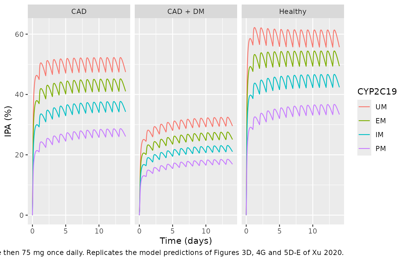
The paper states three quantitative PD results for the 300 mg loading dose followed by 75 mg once daily, and the maintenance doses that restore the IPA of CAD EM patients. It does not say at what time it read IPA off Figures 4G and 5E. The comparison below uses the steady-state trough 24 h after the 14th dose (336 h). At the day-7 trough the ratio and difference claims agree equally well (62.1, 22.1 and 12.7). The dose-adjusted arms are then still 2.4-4.4 IPA points below the reference, because a larger maintenance dose takes longer to approach its steady state.

ipa7 <- sim_pd |>
  filter(time == 336) |>
  select(population, phenotype, md, IPA)
ipa <- function(pop, ph, md = 75) ipa7$IPA[ipa7$population == pop & ipa7$phenotype == ph & ipa7$md == md]
pd_claims <- tibble::tribble(
  ~claim, ~paper, ~simulated,
  "CAD: IPA in PM / IPA in EM (x100)", 62, 100 * ipa("CAD", "PM") / ipa("CAD", "EM"),
  "CAD: IPA(UM) - IPA(PM), percentage points", 23.2, ipa("CAD", "UM") - ipa("CAD", "PM"),
  "CAD + DM: IPA(UM) - IPA(PM), percentage points", 13.7, ipa("CAD + DM", "UM") - ipa("CAD + DM", "PM")
)
knitr::kable(pd_claims, digits = 1, caption = "IPA claims from the Xu 2020 Results and Discussion.")

IPA claims from the Xu 2020 Results and Discussion.

claim	paper	simulated
CAD: IPA in PM / IPA in EM (x100)	62.0	63.5
CAD: IPA(UM) - IPA(PM), percentage points	23.2	21.4
CAD + DM: IPA(UM) - IPA(PM), percentage points	13.7	12.7

dose_up <- tibble::tribble(
  ~scenario,                          ~IPA,
  "CAD EM, 75 mg (reference)",        ipa("CAD", "EM"),
  "CAD PM, 150 mg",                   ipa("CAD", "PM", 150),
  "CAD + DM EM, 150 mg",              ipa("CAD + DM", "EM", 150),
  "CAD + DM IM, 187.5 mg",            ipa("CAD + DM", "IM", 187.5),
  "CAD + DM PM, 265.5 mg",            ipa("CAD + DM", "PM", 265.5)
)
knitr::kable(
  dose_up, digits = 1,
  caption = paste(
    "Maintenance doses that the paper reports restore the IPA of CAD EM",
    "patients on 75 mg (Figures 4G and 5E)."
  )
)

Maintenance doses that the paper reports restore the IPA of CAD EM patients on 75 mg (Figures 4G and 5E).

scenario	IPA
CAD EM, 75 mg (reference)	41.0
CAD PM, 150 mg	40.7
CAD + DM EM, 150 mg	39.4
CAD + DM IM, 187.5 mg	39.2
CAD + DM PM, 265.5 mg	40.8

stopifnot(
  abs(pd_claims$simulated[1] - 62) < 4,
  abs(pd_claims$simulated[2] - 23.2) < 2.5,
  abs(pd_claims$simulated[3] - 13.7) < 2.5,
  # every adjusted dose lands within 2.5 IPA points of the CAD EM reference
  all(abs(dose_up$IPA[-1] - dose_up$IPA[1]) < 2.5)
)

Sensitivity: which DM change lowers CLOP-AM exposure (Figure 7F)

The paper switched each DM change on one at a time in a CAD EM patient after a 300 mg dose. The transit change raised CLOP-AM exposure by 58%. The CES1, CYP2C19 and CYP3A4 changes lowered it by 43%, 24% and 12%. Here each change is isolated by setting the other DM multipliers back to their healthy values through params.

th <- rxode2::rxode(mod)$theta
dm_neutral <- c(e_dm_cyp1a2 = 1, e_dm_cyp2b6 = 1, e_dm_cyp2c9 = 1,
                e_dm_cyp2c19 = 1, e_dm_cyp3a4 = 1, e_dm_ces1 = 1)
transit_healthy <- c(ktr_stomach_dm = th[["ktr_stomach"]], ktr_duodenum_dm = th[["ktr_duodenum"]],
                     ktr_jejunum_dm = th[["ktr_jejunum"]], ktr_ileum_dm = th[["ktr_ileum"]],
                     ktr_cecum_dm = th[["ktr_cecum"]], ktr_colon_dm = th[["ktr_colon"]])
scenarios <- list(
  "Transit rates" = dm_neutral,
  "CES1" = replace(c(dm_neutral, transit_healthy), "e_dm_ces1", th[["e_dm_ces1"]]),
  "CYP2C19" = replace(c(dm_neutral, transit_healthy), "e_dm_cyp2c19", th[["e_dm_cyp2c19"]]),
  "CYP3A4" = replace(c(dm_neutral, transit_healthy), "e_dm_cyp3a4", th[["e_dm_cyp3a4"]])
)
ev_cad <- make_subject(1, "CAD", 0, 300, IHD = 1, obs_times = seq(0, 24, by = 0.02))
auc_h4 <- function(s) {
  sum(diff(s$time) * (head(s$Cc_h4, -1) + tail(s$Cc_h4, -1)) / 2)
}
auc_ref <- auc_h4(solve_typical(ev_cad))
ev_dm <- mutate(ev_cad, DIS_DIAB = 1L)
fig7f <- tibble::tibble(
  change = names(scenarios),
  paper = c(58, -43, -24, -12),
  simulated = vapply(scenarios, function(p) {
    full <- th
    full[names(p)] <- p
    100 * (auc_h4(solve_typical(ev_dm, params = full)) / auc_ref - 1)
  }, numeric(1))
)
knitr::kable(fig7f, digits = 1,
             caption = "Percent change in CLOP-AM AUC0-24 from each isolated DM change (Figure 7F).")

Percent change in CLOP-AM AUC0-24 from each isolated DM change (Figure 7F).

change	paper	simulated
Transit rates	58	57.2
CES1	-43	-45.8
CYP2C19	-24	-23.8
CYP3A4	-12	-11.2

stopifnot(all(abs(fig7f$simulated - fig7f$paper) < 4))

Assumptions and deviations

• Metabolites are formed 1:1 by mass. Equations 13 and 15 add the metabolized clopidogrel (or 2-oxo-CLOP) amount directly to the metabolite with no molecular-weight ratio. The packaged model keeps that as-run form: its states are in mg, and molecular weights are used only to convert concentrations to the molar units of Km (uM) and kirre (mL/nmol/h). A molar-conserving variant that forms CLOP-AM mole-for-mole over-predicts every published CLOP-AM Cmax by a uniform 9% (the 321.82/355.83 molecular-weight ratio). The as-run form reproduces them to within 1.5% after single doses and 3.5% in CAD or after repeated doses. The Kong 2020 vonoprazan code (doi:10.1038/s41401-019-0353-2) from the same group also runs in mass units.
• Molecular weights are not printed in the paper. Clopidogrel 321.82 and CLOP-AM 355.83 g/mol are taken from Jung 2024 (doi:10.1002/psp4.13053). 2-oxo-clopidogrel (C16H16ClNO3S) is 321.82 + 16.00 = 337.82 g/mol.
• Stomach-wall Kt/p is not printed. Table 2 has no stomach row, but the liver equation needs K_st/b. The gut value is used for all three analytes. The stomach wall is a 0.15 L non-eliminating tissue, so this choice has a negligible effect on plasma concentrations.
• The cecum and colon do not absorb. The paper gives Ka,i and Kb,i (and radii) only for the duodenum, jejunum and ileum.
• The liver sums the gut-wall flows over i = 1..5. Eq 11 prints sum(i = 0..5) next to a separate stomach term. Summing i = 1..5 plus the stomach closes the Table 1 flows exactly on the 5.27 L/min cardiac output, so the i = 0 term would double-count the stomach.
• Lung, venous and arterial blood pools are the standard whole-body closure (lung between venous and arterial blood at cardiac output). The paper does not print them; the equations follow Kong 2020 from the same group.
• CLint,CES1,CLOP is in L/h. The paper prints “276,650 1/h”. The 85% share of total intrinsic clearance that the paper cites holds only in L/h (86% with the Table 3 kinetics).
• Enzyme content multiplies Vmax. Eq 12 writes Vmax in pmol/min/pmol P450; the Table 3 enzyme content (pmol P450/mg protein) converts it to a per-mg-protein rate before PBSF scales it to the liver. The same 85% check confirms this.
• CAD flows are 0.90 x the healthy flows (Eq 18) rather than the rounded Table 1 ‘CAD’ column. The two agree to the printed precision.
• DM is only defined together with CAD. The paper’s DM cohort is CAD + DM, whose kirre equals the CAD value. DIS_DIAB = 1 with DIS_IHD = 0 is outside the paper’s scenarios.
• AUC window. Table 4 does not state the AUC window of its predictions. AUC0-6 h reproduces the clopidogrel values and AUC0-5 h the CLOP-AM values, and the partial AUCs in the tables use those windows. The windows are inferred, so the gates use Cmax only; AUC0-24 is shown separately.
• No IIV or residual error. The paper estimated variances for its visual predictive check but did not report them. The model is typical-value only, and the residual SDs are fixed at zero.