Inotuzumab ozogamicin (Garrett 2019)
Source:vignettes/articles/Garrett_2019_inotuzumab.Rmd
Garrett_2019_inotuzumab.RmdModel and source
- Citation: Garrett M, Ruiz-Garcia A, Parivar K, Hee B, Boni J. Population pharmacokinetics of inotuzumab ozogamicin in relapsed/refractory acute lymphoblastic leukemia and non-Hodgkin lymphoma. J Pharmacokinet Pharmacodyn. 2019;46(3):211-222. doi:10.1007/s10928-018-9614-9
- Description: Two-compartment population PK model for inotuzumab ozogamicin in adults with relapsed/refractory B-cell acute lymphoblastic leukemia (ALL) or B-cell non-Hodgkin lymphoma (NHL); linear plus empirical time-dependent (target-mediated) clearance with baseline body surface area on CL1, CL2 and V1, baseline percentage of peripheral-blood blasts on the time-dependent decay coefficient, and concomitant rituximab on CL1 (Garrett 2019, 11 pooled adult studies).
- Article: https://doi.org/10.1007/s10928-018-9614-9 (open access)
- Supplement (Online Resources 1-9, including the final-model NONMEM control stream as Online Resource 3): https://static-content.springer.com/esm/art%3A10.1007%2Fs10928-018-9614-9/MediaObjects/10928_2018_9614_MOESM1_ESM.docx
Inotuzumab ozogamicin (InO) is an anti-CD22 antibody-drug conjugate
carrying N-acetyl-gamma-calicheamicin dimethyl hydrazide. Garrett 2019
pooled 11 adult studies to describe its disposition with a
two-compartment model whose clearance has a constant linear
component (cl_exp_inf, CL1 in the paper) plus an
empirical time-dependent component that decays exponentially
from an initial value (cl_exp_component, CL2) at rate
cl_exp_kdes (kdes):
The decaying arm stands in for target-mediated disposition: as InO
depletes CD22-bearing B cells the target sink shrinks, so clearance
falls toward the linear (catabolic IgG) asymptote. The paper is the
adult predecessor of the pooled adult + pediatric reanalysis packaged as
Wu_2024_inotuzumab.
This vignette is a validation vignette: it checks the packaged model against the numbers Garrett 2019 published, and every check below is a live assertion that fails the render if it stops holding.
Population
The analysis dataset (cutoff 8 March 2016) held 8361 serum InO concentrations from 765 patients across 11 studies: 2 studies of single-agent InO in relapsed or refractory (R/R) B-cell acute lymphoblastic leukemia (ALL, n = 234), and in R/R B-cell non-Hodgkin lymphoma (NHL, n = 531) 3 studies of single-agent InO, 5 of InO plus rituximab, and 1 of InO plus rituximab and chemotherapy (Online Resource 1). Median baseline age was 61 years (range 18-92) and median baseline body surface area 1.84 m^2 (range 1.13-2.81); 40.1% were women and 69.8% were White (Table 1 and Online Resource 4). ALL patients were younger (median 46 vs 65 years) and had higher creatinine clearance (122 vs 82 mL/min) than NHL patients.
Two bioanalytical methods were used, each exclusively within one
tumour type – HPLC/MS/MS (LLOQ 1.0 ng/mL) for the ALL studies and ELISA
(LLOQ 50-667 ng/mL) for the NHL studies. The paper is explicit that its
“ALL effect” therefore confounds disease with assay and cannot be
decomposed; the packaged model carries that caveat in the
DIS_BCPALL covariate metadata.
The same information is available programmatically via the model’s
population metadata
(readModelDb("Garrett_2019_inotuzumab")()$population).
pop <- rxode2::rxode(readModelDb("Garrett_2019_inotuzumab"))$population
#> ℹ parameter labels from comments will be replaced by 'label()'
str(pop[c("n_subjects", "n_studies", "n_observations", "bsa_median")])
#> List of 4
#>  $ n_subjects    : int 765
#>  $ n_studies     : int 11
#>  $ n_observations: int 8361
#>  $ bsa_median    : chr "1.84 m^2 (Garrett 2019 Table 1; the reference value used in every BSA covariate term)"
Source trace
Per-parameter origins are recorded as in-file comments next to each
ini() entry in
inst/modeldb/specificDrugs/Garrett_2019_inotuzumab.R.
Collected here for review. “OR3” is Online Resource 3, the deposited
final-model NONMEM control stream.
| Equation / parameter | Value | Source location |
|---|---|---|
lcl_exp_inf (CL1) |
0.113 L/h | Table 2, “CL 1, L/h” |
lvc (V1) |
6.70 L | Table 2, “V 1, L” |
lcl_exp_component (CL2) |
0.369 L/h | Table 2, “CL 2, L/h” |
lcl_exp_kdes (kdes) |
0.0337 1/h | Table 2, “k des, h-1” |
lq (Q) |
0.0405 L/h | Table 2, “Q, L/h” |
lvp (V2) |
5.10 L | Table 2, “V 2, L” |
e_bsa_cl_exp_inf |
1.54 | Table 2, “CL1 / BBSA effect”; OR3 CL1BBSA
|
e_bsa_cl_exp_component |
1.64 | Table 2, “CL2 / BBSA effect”; OR3 CL2BBSA
|
e_bsa_vc |
0.774 | Table 2, “V1 / BBSA effect”; OR3 V1BBSA (linear, not
power) |
e_all_cl_exp_inf |
-0.745 | Table 2, “CL1 / ALL effect”; OR3 CLPTST
|
e_all_cl_exp_kdes |
-0.860 | Table 2, “kdes / ALL effect”; OR3 KDPTST
|
e_blstpb_cl_exp_kdes |
-0.0401 | Table 2, “kdes / BLSTPB effect”; OR3 KDESBLSTPB
|
e_ritux_cl_exp_inf |
0.155 | Table 2, “CL1 / RITX + InO effect”; OR3 CL1RITX
|
| IIV variances (4) | 0.1789 / 0.1697 / 0.4516 / 0.2070 | Table 2 %CV column (42.3 / 41.2 / 67.2 / 45.5) squared, per footnote c |
| IIV covariances (3) | 0.156 / 0.213 / 0.222 | Table 2, “CL1-V1”, “CL1-CL2”, “CL2-V1” |
expSd |
0.619 (ALL); 0.453 (NHL) | Table 2, sigma rows, read as SDs per OR3
$SIGMA 1 FIX
|
d/dt(central), d/dt(peripheral1)
|
n/a | OR3 $DES (K10 = CL/V1,
K12 = Q/V1, K21 = Q/V2,
S1 = V1) |
cl <- cl_exp_inf + cl_exp_component * exp(-cl_exp_kdes * time) |
n/a | Methods, “Base pharmacokinetic model development”; OR3
$DES CL = CL1 + CL2*EXP(-KDES*T)
|
| Reference BSA / BLSTPB | 1.84 m^2 / 5.25% | “Final model results” equation block |
Three readings in that table are not literal transcriptions of Table 2 and are each justified by an independent cross-check; see Reading Table 2 below.
Reading Table 2
Three places where Table 2 as printed is either ambiguous or wrong, and what settles each. The deposited control stream (Online Resource 3) is the arbiter in all three, and in each case the paper’s own reported effect sizes agree with the control stream rather than with the printed label.
# (1) IIV SCALE. Table 2's IIV rows print the *Estimate* on the %CV scale
# (footnote c) while the neighbouring 95% CI columns are on the VARIANCE scale.
# So the variance is CV^2 -- and each one is confirmed by the midpoint of its
# own published CI.
iiv <- tibble::tribble(
  ~param, ~cv_pct, ~ci_lo, ~ci_hi,
  "CL1", 42.3, 0.147, 0.211,
  "V1", 41.2, 0.150, 0.190,
  "CL2", 67.2, 0.370, 0.533,
  "kdes", 45.5, 0.137, 0.277
) |>
  dplyr::mutate(
    variance = (cv_pct / 100)^2,
    ci_mid = (ci_lo + ci_hi) / 2,
    pct_diff = 100 * (variance / ci_mid - 1)
  )
# Deterministic arithmetic on published constants -- no simulation, so a tight
# bound is correct here.
stopifnot(max(abs(iiv$pct_diff)) < 0.5)

# (2) The three published CORRELATIONS (footnote e) are reproduced from those
# variances and the printed covariances, which independently confirms both.
vars <- setNames(iiv$variance, iiv$param)
corrs <- tibble::tribble(
  ~pair, ~covariance, ~published_corr_pct,
  "CL1-V1", 0.156, 89.4,
  "CL1-CL2", 0.213, 75.0,
  "CL2-V1", 0.222, 80.2
) |>
  dplyr::mutate(
    a = c("CL1", "CL1", "CL2"),
    b = c("V1", "CL2", "V1"),
    derived_corr_pct = 100 * covariance / sqrt(vars[a] * vars[b]),
    pct_diff = derived_corr_pct - published_corr_pct
  )
stopifnot(max(abs(corrs$pct_diff)) < 0.2)

knitr::kable(
  iiv |>
    dplyr::select(param, cv_pct, variance, ci_lo, ci_hi, ci_mid) |>
    dplyr::rename(
      "Parameter" = param, "Table 2 %CV" = cv_pct, "Variance = CV^2" = variance,
      "CI lower" = ci_lo, "CI upper" = ci_hi, "CI midpoint" = ci_mid
    ),
  digits = 4,
  caption = "IIV: the Table 2 'Estimate' is a %CV, its CI is a variance; CV^2 lands on the CI midpoint every time."
)| Parameter | Table 2 %CV | Variance = CV^2 | CI lower | CI upper | CI midpoint |
|---|---|---|---|---|---|
| CL1 | 42.3 | 0.1789 | 0.147 | 0.211 | 0.1790 |
| V1 | 41.2 | 0.1697 | 0.150 | 0.190 | 0.1700 |
| CL2 | 67.2 | 0.4516 | 0.370 | 0.533 | 0.4515 |
| kdes | 45.5 | 0.2070 | 0.137 | 0.277 | 0.2070 |
(3) The residual-error rows are standard deviations, not
variances. Table 2 labels them sigma^2 prop /
“Variance of the … population”, but Online Resource 3 fixes
$SIGMA 1 FIX and uses the estimated THETA directly
as the SD:
$ERROR
SIG = THETA(7)                ; prop error for NHL
IF(PTST.EQ.2) SIG = THETA(8)  ; prop error for ALL
IPRED = LOG(F)
W = SIG
Y = IPRED + W*ERR(1)
With ERR(1) ~ N(0, 1), W is the residual SD
on the log scale. The printed 0.453 / 0.619 are therefore SDs, and the
“Variance of” label is a mis-transcription. The successor Wu 2024 refit
reports the same quantities on the same scale (0.444 NHL, 0.612 adult
ALL), which corroborates the SD reading.
And the RITX polarity is printed backwards in
the main text. The equation block glosses RITX as
“(without rituximab) … 1 if applicable”, but Online Resource 3 has
IF(RITX.EQ.1) CL1RITX = 1 ; Most common and
IF(RITX.EQ.0) CL1RITX = (1 + THETA(12)). Both sources
nevertheless agree on the semantics, which is what the model
encodes: absence of rituximab raises CL1 by 15.5%, exactly as the
Results prose states (“the absence of concomitant rituximab use resulted
in an estimated increase of CL1 by 16%”). The check in the next section
pins it numerically.
Structural checks against the published typical-value equations
Garrett 2019 prints the final-model typical-value equations twice – once for an NHL patient and once, with the covariate terms already folded in, for an ALL patient. Reproducing the ALL form from the NHL parameterisation is a strict test of the disease gate, the rituximab polarity and the covariate algebra together.
mod <- readModelDb("Garrett_2019_inotuzumab")
ui <- rxode2::rxode(mod)
#> ℹ parameter labels from comments will be replaced by 'label()'

# Guard: this model must integrate its explicit ODEs. A cl/vc pair can make
# rxode2 substitute an analytic linCmt() solution and silently discard the
# d/dt() block -- which would drop the time-dependent clearance entirely.
stopifnot(is.null(ui$linCmt))
stopifnot(identical(ui$state, c("central", "peripheral1")))

th <- setNames(ui$theta, names(ui$theta))
cl1 <- exp(th[["lcl_exp_inf"]])
kdes <- exp(th[["lcl_exp_kdes"]])

# ALL patients received single-agent InO, so CONMED_RITUX = 0 and the +15.5%
# no-rituximab term applies. Published ALL equations:
#   CL1  = 0.0333 L/h * (BBSA/1.84)^1.54
#   kdes = 0.00472 /h * (BLSTPB/5.25)^-0.0401
cl1_all <- cl1 * (1 + th[["e_all_cl_exp_inf"]]) *
  (1 + th[["e_ritux_cl_exp_inf"]] * (1 - 0))
kdes_all <- kdes * (1 + th[["e_all_cl_exp_kdes"]])

# The published values are rounded to 3 significant figures, so compare with an
# absolute tolerance set by that rounding, not a relative one.
stopifnot(abs(cl1_all - 0.0333) < 5e-5)
stopifnot(abs(kdes_all - 0.00472) < 5e-6)

# Total CL for an ALL patient at reference covariates on Cycle 4 Day 1
# (day 78 after the first dose) -- the paper states 0.0333 L/h, i.e. the
# decaying arm has become negligible by then.
t_c4d1 <- 77 * 24
cl_total_c4d1 <- cl1_all +
  exp(th[["lcl_exp_component"]]) * exp(-kdes_all * t_c4d1)
stopifnot(abs(cl_total_c4d1 - 0.0333) < 5e-5)

tibble::tibble(
  Quantity = c("CL1, ALL (L/h)", "kdes, ALL (1/h)", "Total CL at C4D1 (L/h)"),
  Published = c(0.0333, 0.00472, 0.0333),
  Reproduced = c(cl1_all, kdes_all, cl_total_c4d1)
) |>
knitr::kable(digits = 6, caption = "Published ALL-arm typical values, reproduced from the NHL parameterisation.")| Quantity | Published | Reproduced |
|---|---|---|
| CL1, ALL (L/h) | 0.03330 | 0.033281 |
| kdes, ALL (1/h) | 0.00472 | 0.004718 |
| Total CL at C4D1 (L/h) | 0.03330 | 0.033342 |
Covariate effect magnitudes
The Results section quantifies each retained covariate at the 10th
and 90th percentiles of its distribution. These are deterministic
functions of the published coefficients, so they are checked tightly.
The V1 row is the discriminating one: it is the only
covariate entering linearly in the centered deviation
rather than as a power model, and a power form would miss the published
values by more than a factor of two.
bsa_lo <- 1.55 # 10th percentile
bsa_hi <- 2.21 # 90th percentile
bl_lo <- 0.0001 # 10th percentile of BLSTPB, %
bl_hi <- 69 # 90th percentile of BLSTPB, %

cov_chk <- tibble::tribble(
  ~Parameter, ~Covariate, ~Level, ~Published_pct, ~Model_pct,
  "CL1", "BSA 1.55 m^2", "10th", -23, 100 * ((bsa_lo / 1.84)^th[["e_bsa_cl_exp_inf"]] - 1),
  "CL1", "BSA 2.21 m^2", "90th", 33, 100 * ((bsa_hi / 1.84)^th[["e_bsa_cl_exp_inf"]] - 1),
  "CL2", "BSA 1.55 m^2", "10th", -25, 100 * ((bsa_lo / 1.84)^th[["e_bsa_cl_exp_component"]] - 1),
  "CL2", "BSA 2.21 m^2", "90th", 35, 100 * ((bsa_hi / 1.84)^th[["e_bsa_cl_exp_component"]] - 1),
  "V1", "BSA 1.55 m^2", "10th", -23, 100 * ((1 + th[["e_bsa_vc"]] * (bsa_lo - 1.84)) - 1),
  "V1", "BSA 2.21 m^2", "90th", 29, 100 * ((1 + th[["e_bsa_vc"]] * (bsa_hi - 1.84)) - 1),
  "kdes", "BLSTPB 0.0001%", "10th", 55, 100 * ((bl_lo / 5.25)^th[["e_blstpb_cl_exp_kdes"]] - 1),
  "kdes", "BLSTPB 69%", "90th", -10, 100 * ((bl_hi / 5.25)^th[["e_blstpb_cl_exp_kdes"]] - 1)
) |>
  dplyr::mutate(Difference = Model_pct - Published_pct)

# Published percentages are rounded to whole numbers, so an absolute tolerance
# of 1.5 percentage points is the rounding budget plus a little headroom.
stopifnot(max(abs(cov_chk$Difference)) < 1.5)

# The V1 effect is LINEAR in (BSA - 1.84). Prove the gate discriminates: the
# power-model misreading is wrong by far more than the tolerance above, so this
# check would go red if the model file used the wrong functional form.
v1_power_err <- 100 * ((bsa_hi / 1.84)^th[["e_bsa_vc"]] - 1) - 29
stopifnot(abs(v1_power_err) > 10)

cov_chk |>
  dplyr::select(-Level) |>
  dplyr::rename(
    "Published change (%)" = Published_pct,
    "Model change (%)" = Model_pct,
    "Difference (pp)" = Difference
  ) |>
knitr::kable(digits = 1, caption = "Covariate effect sizes at the 10th and 90th percentiles (Garrett 2019 Results).")| Parameter | Covariate | Published change (%) | Model change (%) | Difference (pp) |
|---|---|---|---|---|
| CL1 | BSA 1.55 m^2 | -23 | -23.2 | -0.2 |
| CL1 | BSA 2.21 m^2 | 33 | 32.6 | -0.4 |
| CL2 | BSA 1.55 m^2 | -25 | -24.5 | 0.5 |
| CL2 | BSA 2.21 m^2 | 35 | 35.1 | 0.1 |
| V1 | BSA 1.55 m^2 | -23 | -22.4 | 0.6 |
| V1 | BSA 2.21 m^2 | 29 | 28.6 | -0.4 |
| kdes | BLSTPB 0.0001% | 55 | 54.6 | -0.4 |
| kdes | BLSTPB 69% | -10 | -9.8 | 0.2 |
Decay of the time-dependent clearance component
kdes_at <- function(blstpb) kdes_all * (blstpb / 5.25)^th[["e_blstpb_cl_exp_kdes"]]
half <- function(k) log(2) / k

# "for patients with ALL, after approximately 147 h (i.e. ln(2)/kdes when
# BLSTPB is 5.25%) ... the contribution of CLt is reduced by 50%"
stopifnot(abs(half(kdes_at(5.25)) - 147) < 1.5)

# "variations in the time corresponding to a 50% reduction in CLt ... ranged
# from 95 to 163 h"
stopifnot(abs(half(kdes_at(bl_lo)) - 95) < 1.5)
stopifnot(abs(half(kdes_at(bl_hi)) - 163) < 1.5)

# "this contribution of CLt on total clearance became negligible after 5
# half-lives ... 2.8 weeks (10th percentile), 4.4 weeks (50th), 4.8 weeks (90th)"
weeks5 <- function(k) 5 * half(k) / (24 * 7)
pub_weeks <- c(2.8, 4.4, 4.8)
mod_weeks <- c(weeks5(kdes_at(bl_lo)), weeks5(kdes_at(5.25)), weeks5(kdes_at(bl_hi)))
stopifnot(max(abs(mod_weeks - pub_weeks)) < 0.06)

tibble::tibble(
  BLSTPB = c("0.0001% (10th)", "5.25% (50th)", "69% (90th)"),
  `kdes (1/h)` = c(kdes_at(bl_lo), kdes_at(5.25), kdes_at(bl_hi)),
  `t1/2 of CLt (h), published` = c(95, 147, 163),
  `t1/2 of CLt (h), model` = c(half(kdes_at(bl_lo)), half(kdes_at(5.25)), half(kdes_at(bl_hi))),
  `5 half-lives (wk), published` = pub_weeks,
  `5 half-lives (wk), model` = mod_weeks
) |>
knitr::kable(digits = c(0, 5, 0, 1, 1, 2), caption = "Timescale of the decaying clearance arm across the BLSTPB range.")| BLSTPB | kdes (1/h) | t1/2 of CLt (h), published | t1/2 of CLt (h), model | 5 half-lives (wk), published | 5 half-lives (wk), model |
|---|---|---|---|---|---|
| 0.0001% (10th) | 0.00730 | 95 | 95.0 | 2.8 | 2.83 |
| 5.25% (50th) | 0.00472 | 147 | 146.9 | 4.4 | 4.37 |
| 69% (90th) | 0.00425 | 163 | 162.9 | 4.8 | 4.85 |
Terminal half-life
Garrett 2019 reports a terminal beta half-life of 293 h (12 days)
from its model-based simulations in ALL patients. Once the decaying arm
has vanished the system is an ordinary two-compartment model, so the
published value is a joint test of CL1, V1,
Q and V2 at once.
v1 <- exp(th[["lvc"]])
q <- exp(th[["lq"]])
v2 <- exp(th[["lvp"]])

k10 <- cl1_all / v1
k12 <- q / v1
k21 <- q / v2
s <- k10 + k12 + k21
beta <- (s - sqrt(s^2 - 4 * k10 * k21)) / 2
t_half_beta <- log(2) / beta

# 293 h is rounded to 3 significant figures; 5 h of tolerance is ~1.7%, which a
# mis-transcribed clearance or volume would blow through many times over.
stopifnot(abs(t_half_beta - 293) < 5)
cat(sprintf("Terminal beta half-life: %.1f h (published 293 h)\n", t_half_beta))
#> Terminal beta half-life: 291.2 h (published 293 h)
Virtual cohort
Original observed data are not publicly available. The cohort below reproduces the three covariate scenarios Garrett 2019 simulated in Figures 7 and 8, for ALL patients on the fixed 1.8 mg/m^2/cycle regimen:
- A – low BSA (1.55 m^2) and low BLSTPB (0.0001%): highest exposure.
- B – median BSA (1.84 m^2) and median BLSTPB (5.25%).
- C – high BSA (2.21 m^2) and high BLSTPB (69%): lowest exposure.
Each scenario fixes its covariates at the stated percentile (as the paper’s simulations did) and carries the model’s full between-subject variability.
# `set.seed()` seeds R's RNG, not rxode2's; rxode2 partitions its streams per
# solver thread, so this cohort differs between a 2-core CI runner and a
# 16-thread workstation. Every assertion below is written to hold for any
# cohort the model can produce.
set.seed(20190311)

n_per_arm <- 200L

# Fractionated regimen: 0.8 mg/m^2 on day 1 and 0.5 mg/m^2 on days 8 and 15 of
# each cycle; cycle 1 lasts 21 days and subsequent cycles 28 days. Times below
# are hours from the first dose (the paper's "day 1"), which is the driver the
# time-dependent clearance consumes.
cycle_start_h <- c(0, 21, 49, 77) * 24 # C1D1, C2D1, C3D1, C4D1
dose_times_h <- sort(as.vector(outer(c(0, 7, 14) * 24, cycle_start_h, "+")))
dose_mg_m2 <- rep(c(0.8, 0.5, 0.5), times = 4)[order(as.vector(outer(c(0, 7, 14) * 24, cycle_start_h, "+")))]
# Drop the doses that fall after the last AUC window closes (C4D1 at 1848 h is
# the right-hand boundary of the day-64 interval and is retained).
keep_dose <- dose_times_h <= 1848
dose_times_h <- dose_times_h[keep_dose]
dose_mg_m2 <- dose_mg_m2[keep_dose]

# Observation grid: dense immediately after each dose so the peaks are resolved
# (an under-sampled Tmax understates AUC by several percent), coarse thereafter.
post_dose_offsets <- c(0, 0.25, 0.5, 0.75, 1, 1.25, 1.5, 2, 3, 4, 6, 9, 12, 18, 24, 36, 48, 72, 96, 120, 144)
obs_times_h <- sort(unique(c(
  as.vector(outer(post_dose_offsets, dose_times_h, "+")),
  seq(0, 1848, by = 12),
  # The three AUC interval boundaries must carry an observation exactly, or
  # PKNCA integrates only as far as the last point inside the window.
  0, 168, 672, 840, 1512, 1848
)))
obs_times_h <- obs_times_h[obs_times_h >= 0 & obs_times_h <= 1848]

scenarios <- tibble::tribble(
  ~scenario, ~BSA_BASE, ~BLSTPB,
  "A: low BSA / low blasts", 1.55, 0.0001,
  "B: median BSA / median blasts", 1.84, 5.25,
  "C: high BSA / high blasts", 2.21, 69
)

make_cohort <- function(n, scenario, BSA_BASE, BLSTPB, id_offset = 0L) {
  subj <- tibble::tibble(
    id = id_offset + seq_len(n),
    scenario = scenario,
    BSA_BASE = BSA_BASE,
    BLSTPB = BLSTPB,
    DIS_BCPALL = 1, # B-cell ALL
    CONMED_RITUX = 0 # single-agent InO in every ALL study
  )
  doses <- subj |>
    tidyr::crossing(tibble::tibble(time = dose_times_h, dose_mg_m2 = dose_mg_m2)) |>
    dplyr::mutate(
      amt = dose_mg_m2 * BSA_BASE,
      evid = 1L,
      cmt = "central",
      # 1-hour intravenous infusion (see Assumptions).
      rate = amt / 1
    ) |>
    dplyr::select(-dose_mg_m2)
  obs <- subj |>
    tidyr::crossing(tibble::tibble(time = obs_times_h)) |>
    dplyr::mutate(amt = NA_real_, evid = 0L, cmt = "central", rate = NA_real_)
  dplyr::bind_rows(doses, obs) |>
    dplyr::arrange(id, time, dplyr::desc(evid))
}

events <- dplyr::bind_rows(
  Map(
    function(s, b, bl, off) make_cohort(n_per_arm, s, b, bl, id_offset = off),
    scenarios$scenario, scenarios$BSA_BASE, scenarios$BLSTPB,
    c(0L, n_per_arm, 2L * n_per_arm)
  )
)

# Disjoint IDs across arms: duplicated IDs are silently merged by rxSolve into a
# single subject receiving the summed dose.
stopifnot(!anyDuplicated(unique(events[, c("id", "time", "evid")])))
stopifnot(dplyr::n_distinct(events$id) == 3L * n_per_arm)
Simulation
sim <- rxode2::rxSolve(
  mod,
  events = events,
  keep = c("scenario", "BSA_BASE", "BLSTPB")
) |>
  as.data.frame()
#> ℹ parameter labels from comments will be replaced by 'label()'

# Fail loudly rather than letting a degenerate solve pass downstream as an
# empty-but-successful NCA.
stopifnot(nrow(sim) > 0, !all(is.na(sim$Cc)), all(sim$Cc >= 0, na.rm = TRUE))
Replicate published figures
# Replicates Figure 7 of Garrett 2019: simulated InO concentration-time course
# in ALL patients at 1.8 mg/m^2/cycle, by covariate scenario. Red (A) is the
# highest-exposure scenario and blue (C) the lowest.
sim |>
  dplyr::filter(!is.na(Cc)) |>
  dplyr::group_by(scenario, time) |>
  dplyr::summarise(
    Q05 = quantile(Cc, 0.05),
    Q50 = median(Cc),
    Q95 = quantile(Cc, 0.95),
    .groups = "drop"
  ) |>
  ggplot(aes(time / 24, Q50, colour = scenario, fill = scenario)) +
  geom_ribbon(aes(ymin = Q05, ymax = Q95), alpha = 0.15, colour = NA) +
  geom_line(linewidth = 0.6) +
  scale_y_log10() +
  scale_colour_manual(values = c("firebrick", "grey30", "steelblue")) +
  scale_fill_manual(values = c("firebrick", "grey30", "steelblue")) +
  labs(
    x = "Time from first dose (days)", y = "InO concentration (ng/mL)",
    colour = NULL, fill = NULL,
    title = "Figure 7 - covariate effects on the InO concentration-time course",
    caption = "Median with 5th-95th percentile band; replicates Figure 7 of Garrett 2019."
  ) +
  theme_bw() +
  theme(legend.position = "bottom")
#> Warning in scale_y_log10(): log-10 transformation introduced infinite values.
#> log-10 transformation introduced infinite values.
#> log-10 transformation introduced infinite values.
#> log-10 transformation introduced infinite values.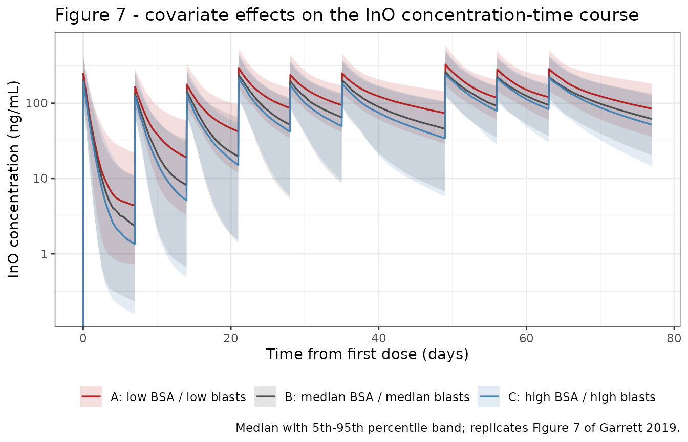
The paper’s reading of this figure is that the highest- and lowest-exposure scenarios “showed substantial overlap in the simulated InO concentrations and exposure”, i.e. the retained covariates are statistically significant but not clinically meaningful. The overlap is checked quantitatively below.
# Companion to Figure 6: accumulation of the pre-dose trough across cycles.
# Trough concentrations immediately before each cycle's day-1 dose.
trough <- sim |>
  dplyr::filter(time %in% cycle_start_h, !is.na(Cc)) |>
  dplyr::group_by(scenario, time) |>
  dplyr::summarise(Q50 = median(Cc), .groups = "drop") |>
  dplyr::mutate(cycle = factor(round(time / 24) + 1))

ggplot(trough, aes(cycle, Q50, colour = scenario, group = scenario)) +
  geom_line() +
  geom_point() +
  scale_x_discrete(labels = c("C1D1", "C2D1", "C3D1", "C4D1")) +
  labs(
    x = "Cycle day-1 (pre-dose)", y = "Median trough InO (ng/mL)", colour = NULL,
    title = "Trough accumulation across four cycles",
    caption = "Cycle 1 is 21 days and later cycles 28 days, so the C2D1 trough follows a 7-day gap and the C3D1 / C4D1 troughs a 14-day gap."
  ) +
  theme_bw() +
  theme(legend.position = "bottom")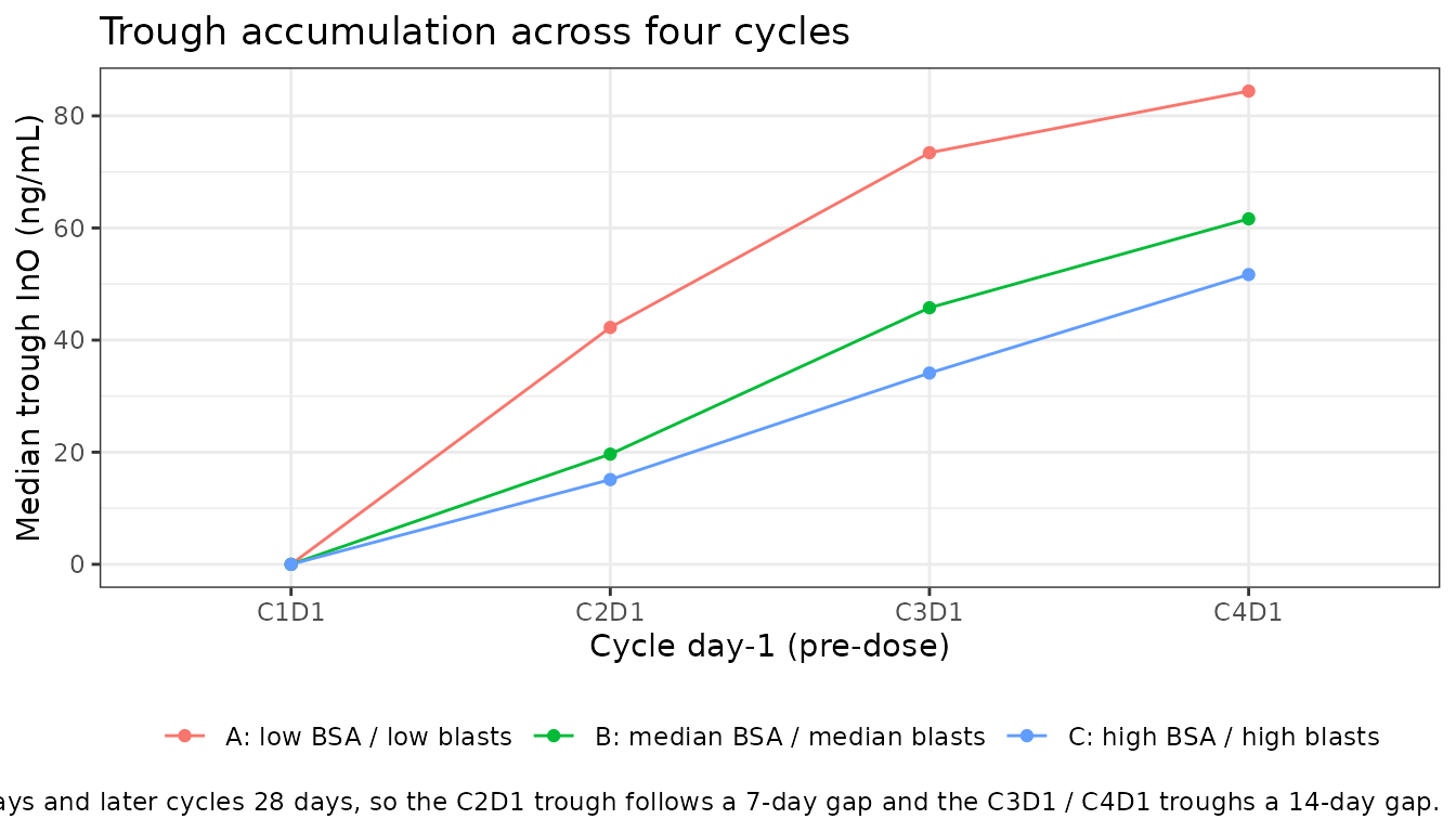
# Troughs accumulate monotonically in every arm. This is the only claim the
# trough series can carry on its own: cycle 1 is 21 days and later cycles are
# 28 days, so the C2D1 trough follows a 7-day washout while C3D1 and C4D1
# follow 14-day washouts. Increments across that boundary are not comparable,
# and the paper's steady-state claim is therefore tested on dose- and
# tau-normalised AUCtau instead (see "Approach to steady state" below), which
# is the quantity Garrett 2019 actually reports.
mono <- trough |>
  dplyr::arrange(scenario, time) |>
  dplyr::group_by(scenario) |>
  dplyr::summarise(increasing = all(diff(Q50) > 0), .groups = "drop")
stopifnot(nrow(mono) == 3L, all(mono$increasing))
PKNCA validation
Figure 8 of Garrett 2019 reports the median simulated AUCtau at three timepoints, for each of the three covariate scenarios – nine published values. The dosing interval differs by timepoint (7 days on days 1 and 29; 14 days on day 64, because the day-64 dose is the last of cycle 3 and the next dose is cycle 4 day 1 on day 78). Note that “day n” in the paper is 1-indexed from the first dose, so day 29 is 28 days = 672 h after time zero.
# Only !is.na(Cc) -- a `time > 0` or `Cc > 0` filter would drop the time-zero
# anchor and trigger PKNCA's "AUC range starting (0) before the first
# measurement" warning once per subject.
sim_nca <- sim |>
  dplyr::filter(!is.na(Cc)) |>
  dplyr::select(id, time, Cc, scenario)

# Guarantee a time-zero row per subject. InO is given intravenously and these
# are treatment-naive first doses, so pre-dose Cc = 0 is correct.
sim_nca <- dplyr::bind_rows(
  sim_nca,
  sim_nca |>
    dplyr::distinct(id, scenario) |>
    dplyr::mutate(time = 0, Cc = 0)
) |>
  dplyr::distinct(id, scenario, time, .keep_all = TRUE) |>
  dplyr::arrange(id, scenario, time)

stopifnot(nrow(sim_nca) > 0)
stopifnot(all(tapply(sim_nca$time, sim_nca$id, min) == 0))

dose_df <- events |>
  dplyr::filter(evid == 1) |>
  dplyr::select(id, time, amt, scenario)

conc_obj <- PKNCA::PKNCAconc(
  sim_nca, Cc ~ time | scenario + id,
  concu = "ng/mL", timeu = "h"
)
dose_obj <- PKNCA::PKNCAdose(dose_df, amt ~ time | scenario + id, doseu = "mg")

intervals <- data.frame(
  start = c(0, 672, 1512),
  end = c(168, 840, 1848),
  cmax = c(TRUE, FALSE, FALSE),
  tmax = c(TRUE, FALSE, FALSE),
  auclast = TRUE
)

nca_res <- PKNCA::pk.nca(PKNCA::PKNCAdata(conc_obj, dose_obj, intervals = intervals))

nca_tbl <- as.data.frame(nca_res$result) |>
  dplyr::filter(PPTESTCD == "auclast") |>
  dplyr::mutate(
    timepoint = dplyr::case_when(
      start == 0 ~ "Day 1 (0.8 mg/m2, tau 7 d)",
      start == 672 ~ "Day 29 (0.5 mg/m2, tau 7 d)",
      start == 1512 ~ "Day 64 (0.5 mg/m2, tau 14 d)"
    )
  )
stopifnot(nrow(nca_tbl) == 3L * 3L * n_per_arm)
Comparison against published NCA
published <- tibble::tribble(
  ~scenario, ~timepoint, ~auclast,
  "A: low BSA / low blasts", "Day 1 (0.8 mg/m2, tau 7 d)", 4550,
  "B: median BSA / median blasts", "Day 1 (0.8 mg/m2, tau 7 d)", 3790,
  "C: high BSA / high blasts", "Day 1 (0.8 mg/m2, tau 7 d)", 3380,
  "A: low BSA / low blasts", "Day 29 (0.5 mg/m2, tau 7 d)", 22800,
  "B: median BSA / median blasts", "Day 29 (0.5 mg/m2, tau 7 d)", 17100,
  "C: high BSA / high blasts", "Day 29 (0.5 mg/m2, tau 7 d)", 14300,
  "A: low BSA / low blasts", "Day 64 (0.5 mg/m2, tau 14 d)", 44700,
  "B: median BSA / median blasts", "Day 64 (0.5 mg/m2, tau 14 d)", 37600,
  "C: high BSA / high blasts", "Day 64 (0.5 mg/m2, tau 14 d)", 32400
)

simulated_median <- nca_tbl |>
  dplyr::group_by(scenario, timepoint) |>
  dplyr::summarise(simulated = median(PPORRES), .groups = "drop")

cmp <- published |>
  dplyr::left_join(simulated_median, by = c("scenario", "timepoint")) |>
  dplyr::mutate(pct_diff = 100 * (simulated / auclast - 1))

stopifnot(nrow(cmp) == 9L, !anyNA(cmp$simulated))

cmp |>
  dplyr::mutate(flag = ifelse(abs(pct_diff) > 20, "*", "")) |>
  dplyr::select(timepoint, scenario, auclast, simulated, pct_diff, flag) |>
  dplyr::rename(
    "Timepoint" = timepoint,
    "Scenario" = scenario,
    "Published median AUCtau (ng*h/mL)" = auclast,
    "Simulated median AUCtau (ng*h/mL)" = simulated,
    "% diff" = pct_diff,
    " " = flag
  ) |>
  knitr::kable(
    digits = c(0, 0, 0, 0, 1, 0),
    caption = "Simulated vs. Figure 8 of Garrett 2019. * differs from the published median by >20%."
)| Timepoint | Scenario | Published median AUCtau (ng*h/mL) | Simulated median AUCtau (ng*h/mL) | % diff | |
|---|---|---|---|---|---|
| Day 1 (0.8 mg/m2, tau 7 d) | A: low BSA / low blasts | 4550 | 4779 | 5.0 | |
| Day 1 (0.8 mg/m2, tau 7 d) | B: median BSA / median blasts | 3790 | 3959 | 4.5 | |
| Day 1 (0.8 mg/m2, tau 7 d) | C: high BSA / high blasts | 3380 | 3423 | 1.3 | |
| Day 29 (0.5 mg/m2, tau 7 d) | A: low BSA / low blasts | 22800 | 23380 | 2.5 | |
| Day 29 (0.5 mg/m2, tau 7 d) | B: median BSA / median blasts | 17100 | 17569 | 2.7 | |
| Day 29 (0.5 mg/m2, tau 7 d) | C: high BSA / high blasts | 14300 | 14308 | 0.1 | |
| Day 64 (0.5 mg/m2, tau 14 d) | A: low BSA / low blasts | 44700 | 46756 | 4.6 | |
| Day 64 (0.5 mg/m2, tau 14 d) | B: median BSA / median blasts | 37600 | 37223 | -1.0 | |
| Day 64 (0.5 mg/m2, tau 14 d) | C: high BSA / high blasts | 32400 | 34305 | 5.9 |
# The published values are medians of a 1000-subject simulation; this vignette
# draws 200 per arm on a machine-dependent RNG partition, so the comparison is
# between two cohort medians and needs headroom. Realised |%diff| across all
# nine cells on the authoring machine: max 5.9, median 2.7. 20% still goes red
# on a mis-transcribed dose, clearance, BSA exponent or the mg -> ng/mL
# scaling, each of which moves AUC by tens of percent.
stopifnot(max(abs(cmp$pct_diff)) < 20)
# Centre of the distribution: a structural error shifts every cell one way.
stopifnot(abs(median(cmp$pct_diff)) < 10)

# The covariate ORDERING is the qualitative claim of Figure 8 (A > B > C at
# every timepoint) and is a large, reproducible effect -- A/C differ by ~35-60%,
# far outside cohort noise.
ord <- cmp |>
  dplyr::group_by(timepoint) |>
  dplyr::summarise(
    ok = simulated[startsWith(scenario, "A")] > simulated[startsWith(scenario, "B")] &&
      simulated[startsWith(scenario, "B")] > simulated[startsWith(scenario, "C")],
    .groups = "drop"
  )
stopifnot(nrow(ord) == 3L, all(ord$ok))
Approach to steady state
Garrett 2019 states that “steady-state levels were achieved after 3 cycles of treatment following multiple dosing.” The three Figure 8 timepoints differ in both dose (0.8 mg/m^2 on day 1, 0.5 mg/m^2 on days 29 and 64) and dosing interval (7 days on days 1 and 29, 14 days on day 64), so the comparable quantity is AUCtau divided by tau and by the dose – exposure per unit time per unit dose. On that scale the paper’s own published medians rise about seven-fold from day 1 to day 29 and then change by roughly a tenth to day 64, which is what “steady state by cycle 3” means here. The packaged model reproduces both legs.
tau_h <- c(
  "Day 1 (0.8 mg/m2, tau 7 d)" = 168,
  "Day 29 (0.5 mg/m2, tau 7 d)" = 168,
  "Day 64 (0.5 mg/m2, tau 14 d)" = 336
)
dose_m2 <- c(
  "Day 1 (0.8 mg/m2, tau 7 d)" = 0.8,
  "Day 29 (0.5 mg/m2, tau 7 d)" = 0.5,
  "Day 64 (0.5 mg/m2, tau 14 d)" = 0.5
)

norm <- cmp |>
  dplyr::mutate(
    published_norm = auclast / tau_h[timepoint] / dose_m2[timepoint],
    simulated_norm = simulated / tau_h[timepoint] / dose_m2[timepoint]
  )

ratios <- norm |>
  dplyr::group_by(scenario) |>
  dplyr::summarise(
    pub_d29_d1 = published_norm[startsWith(timepoint, "Day 29")] /
      published_norm[startsWith(timepoint, "Day 1")],
    sim_d29_d1 = simulated_norm[startsWith(timepoint, "Day 29")] /
      simulated_norm[startsWith(timepoint, "Day 1")],
    pub_d64_d29 = published_norm[startsWith(timepoint, "Day 64")] /
      published_norm[startsWith(timepoint, "Day 29")],
    sim_d64_d29 = simulated_norm[startsWith(timepoint, "Day 64")] /
      simulated_norm[startsWith(timepoint, "Day 29")],
    .groups = "drop"
  )

# Leg 1 -- large, unambiguous accumulation from cycle 1 to cycle 2/3. Published
# 6.8-8.0x, simulated 6.7-7.8x on the authoring machine. A 4x floor is far
# below either and is not reachable without accumulation.
stopifnot(all(ratios$pub_d29_d1 > 4), all(ratios$sim_d29_d1 > 4))

# Leg 2 -- the plateau. Published 0.98-1.13x, simulated 1.00-1.20x. The band
# below admits both while still rejecting continued accumulation at the leg-1
# rate, which would land near 2x or beyond.
stopifnot(all(ratios$pub_d64_d29 > 0.85 & ratios$pub_d64_d29 < 1.35))
stopifnot(all(ratios$sim_d64_d29 > 0.85 & ratios$sim_d64_d29 < 1.35))

# And the model tracks the paper arm by arm, not merely inside the same band.
# Largest realised discrepancy 0.066; 0.20 leaves room for cohort noise.
stopifnot(max(abs(ratios$sim_d64_d29 - ratios$pub_d64_d29)) < 0.20)

ratios |>
  dplyr::rename(
    "Scenario" = scenario,
    "Day 29 / Day 1, published" = pub_d29_d1,
    "Day 29 / Day 1, model" = sim_d29_d1,
    "Day 64 / Day 29, published" = pub_d64_d29,
    "Day 64 / Day 29, model" = sim_d64_d29
  ) |>
  knitr::kable(
    digits = 2,
    caption = "Dose- and tau-normalised AUCtau ratios: a ~7-fold rise to cycle 3, then a plateau."
)| Scenario | Day 29 / Day 1, published | Day 29 / Day 1, model | Day 64 / Day 29, published | Day 64 / Day 29, model |
|---|---|---|---|---|
| A: low BSA / low blasts | 8.02 | 7.83 | 0.98 | 1.00 |
| B: median BSA / median blasts | 7.22 | 7.10 | 1.10 | 1.06 |
| C: high BSA / high blasts | 6.77 | 6.69 | 1.13 | 1.20 |
# Cmax and Tmax after the first dose, for context. Tmax should sit at the end of
# the 1-hour infusion.
first_dose <- as.data.frame(nca_res$result) |>
  dplyr::filter(start == 0, PPTESTCD %in% c("cmax", "tmax")) |>
  dplyr::group_by(scenario, PPTESTCD) |>
  dplyr::summarise(median = median(PPORRES), .groups = "drop") |>
  tidyr::pivot_wider(names_from = PPTESTCD, values_from = median)

stopifnot(all(first_dose$tmax == 1))

first_dose |>
  dplyr::rename("Scenario" = scenario, "Median Cmax (ng/mL)" = cmax, "Median Tmax (h)" = tmax) |>
knitr::kable(digits = 1, caption = "First-dose Cmax and Tmax by scenario (not reported in Garrett 2019; shown for context).")| Scenario | Median Cmax (ng/mL) | Median Tmax (h) |
|---|---|---|
| A: low BSA / low blasts | 248.9 | 1 |
| B: median BSA / median blasts | 202.1 | 1 |
| C: high BSA / high blasts | 193.3 | 1 |
Exposure overlap across covariate scenarios
# "Patients with the highest exposure ... and lowest exposure ... showed
# substantial overlap in the simulated InO concentrations and exposure."
# Operationalised as: the interquartile ranges of the A and C arms overlap at
# every timepoint. Quantile overlap between two 200-subject samples whose
# medians differ by ~35% is a stable, large-margin comparison.
overlap <- nca_tbl |>
  dplyr::filter(startsWith(scenario, "A") | startsWith(scenario, "C")) |>
  dplyr::group_by(timepoint, arm = substr(scenario, 1, 1)) |>
  dplyr::summarise(q25 = quantile(PPORRES, 0.25), q75 = quantile(PPORRES, 0.75), .groups = "drop") |>
  tidyr::pivot_wider(names_from = arm, values_from = c(q25, q75))

stopifnot(all(overlap$q25_A < overlap$q75_C))

overlap |>
  dplyr::rename(
    "Timepoint" = timepoint,
    "A: 25th pct" = q25_A, "A: 75th pct" = q75_A,
    "C: 25th pct" = q25_C, "C: 75th pct" = q75_C
  ) |>
knitr::kable(digits = 0, caption = "AUCtau interquartile ranges for the highest- (A) and lowest-exposure (C) scenarios: every A range overlaps its C range.")| Timepoint | A: 25th pct | C: 25th pct | A: 75th pct | C: 75th pct |
|---|---|---|---|---|
| Day 1 (0.8 mg/m2, tau 7 d) | 3280 | 2263 | 7298 | 5588 |
| Day 29 (0.5 mg/m2, tau 7 d) | 18338 | 9223 | 31182 | 21728 |
| Day 64 (0.5 mg/m2, tau 14 d) | 34663 | 22964 | 60498 | 47267 |
Disease effect: ALL versus NHL
The two largest covariate effects in the model are the disease/assay indicators. Garrett 2019 states that in ALL patients “CL1 decreased by 75% (95% CI 71-78%) and kdes decreased by 86% (95% CI 82-90%) relative to patients with B-cell NHL”.
disease <- tibble::tibble(
  Parameter = c("CL1", "kdes"),
  `Published decrease (%)` = c(75, 86),
  `Model decrease (%)` = c(
    -100 * th[["e_all_cl_exp_inf"]],
    -100 * th[["e_all_cl_exp_kdes"]]
  )
) |>
  dplyr::mutate(Difference = `Model decrease (%)` - `Published decrease (%)`)

stopifnot(max(abs(disease$Difference)) < 1)
knitr::kable(disease, digits = 1, caption = "Disease/assay effect on clearance parameters.")| Parameter | Published decrease (%) | Model decrease (%) | Difference |
|---|---|---|---|
| CL1 | 75 | 74.5 | -0.5 |
| kdes | 86 | 86.0 | 0.0 |
# A typical-value comparison of total clearance over time in the two disease
# strata at reference covariates. Both strata share the same CL2 (0.369 L/h --
# no covariate acts on it besides BSA), so the two curves start close together
# and are separated only by the ~3.4-fold difference in the CL1 asymptote. The
# ALL arm's kdes is about seven times smaller, so its decaying component
# persists for weeks while the NHL one is spent within a day or two. The
# consequence is that the curves CROSS twice, which the gate below pins.
tt <- seq(0, 1848, by = 6)
cl_curve <- function(is_all) {
  cl1_i <- cl1 * (1 + th[["e_all_cl_exp_inf"]] * is_all) *
    (1 + th[["e_ritux_cl_exp_inf"]] * (1 - ifelse(is_all == 1, 0, 1)))
  kdes_i <- kdes * (1 + th[["e_all_cl_exp_kdes"]] * is_all)
  cl1_i + exp(th[["lcl_exp_component"]]) * exp(-kdes_i * tt)
}
tibble::tibble(
  time = rep(tt, 2),
  CL = c(cl_curve(0), cl_curve(1)),
  Disease = rep(c("B-cell NHL (+ rituximab)", "B-cell ALL (single agent)"), each = length(tt))
) |>
  ggplot(aes(time / 24, CL, colour = Disease)) +
  geom_line(linewidth = 0.7) +
  scale_y_log10() +
  labs(
    x = "Time from first dose (days)", y = "Total clearance (L/h)", colour = NULL,
    title = "Time-dependent clearance by disease stratum, reference covariates",
    caption = "CL(t) = CL1 + CL2 * exp(-kdes * t); Garrett 2019 Table 2 typical values."
  ) +
  theme_bw() +
  theme(legend.position = "bottom")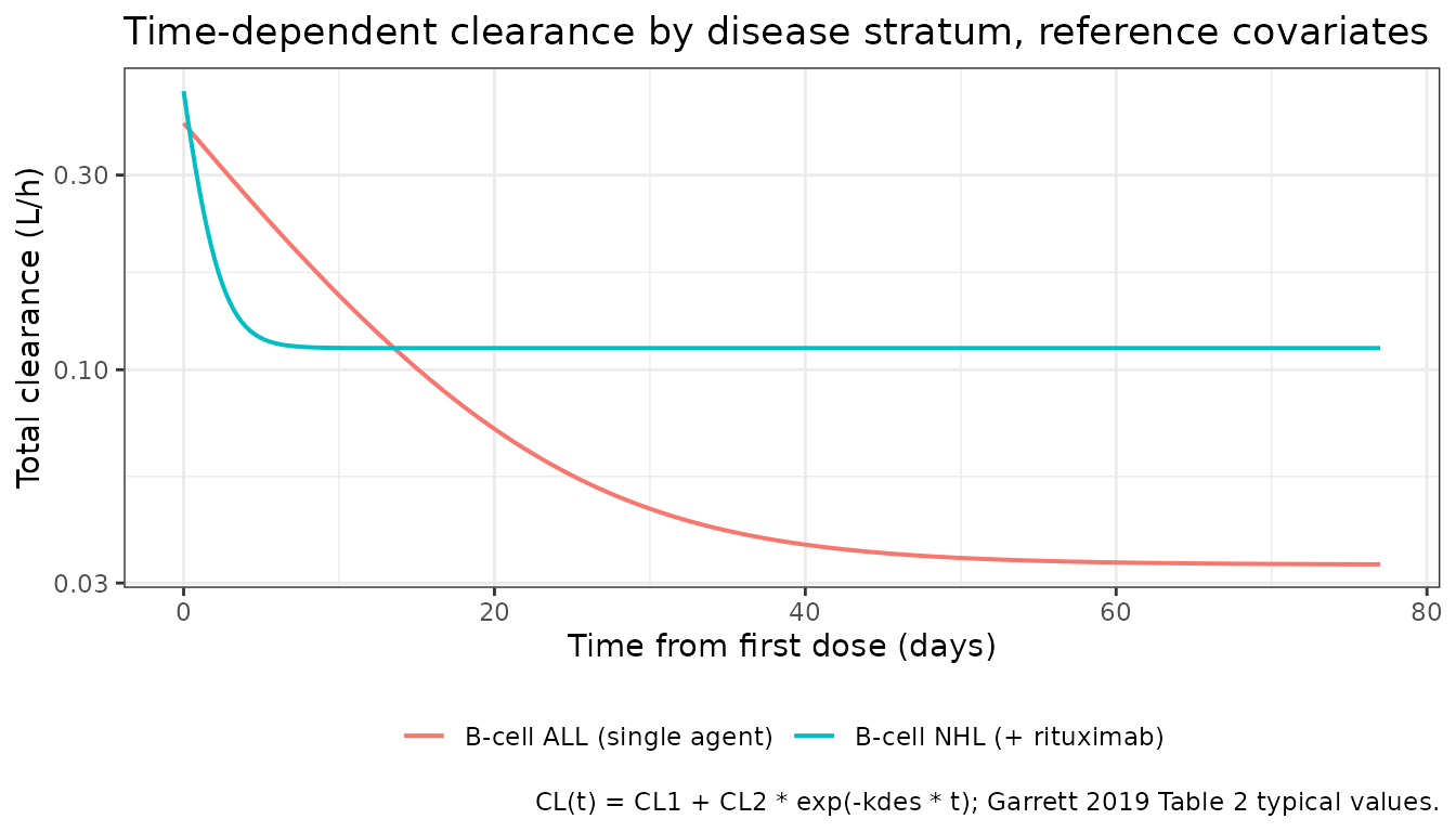
# Everything here is deterministic arithmetic on the published typical values,
# so the tolerances are set by the structure, not by cohort noise.
all_curve <- cl_curve(1)
nhl_curve <- cl_curve(0)

# Both curves decay monotonically to their CL1 asymptote from above. The NHL
# curve is only NON-increasing, not strictly decreasing: past about day 46 its
# decaying term (0.369 * exp(-0.0337 t)) underflows below the last representable
# bit of 0.113, so consecutive grid values are bitwise equal. That is a property
# of double-precision arithmetic, not of the model, and asserting a strict
# decrease here would fail on any machine.
stopifnot(all(diff(all_curve) < 0), all(diff(nhl_curve) <= 0))
stopifnot(all(all_curve > cl1_all), all(nhl_curve >= cl1))

# The NHL decaying arm is spent long before day 77 (kdes = 0.0337/h gives a
# ~21 h half-life), so that curve has reached its asymptote to machine
# precision.
stopifnot(abs(tail(nhl_curve, 1) - cl1) < 1e-6)

# The ALL arm has NOT: its kdes is ~7x smaller (147 h half-life), so at day 77
# a small remnant of CL2 is still present. It is under 1% of the asymptote --
# which is why the paper can quote 0.0333 L/h as the ALL typical CL at C4D1 --
# but it is far above 1e-6 and asserting otherwise would be wrong.
all_remnant <- (tail(all_curve, 1) - cl1_all) / cl1_all
stopifnot(all_remnant > 0, all_remnant < 0.01)

# The curves CROSS TWICE. They start together (same CL2) with NHL above by the
# CL1 difference; the NHL decaying arm then collapses while the ALL one lingers,
# putting ALL on top through the middle weeks; finally the ALL arm decays too
# and the CL1 asymptotes restore the NHL-above ordering. Two sign changes, no
# more -- a wrong kdes gate or a lost disease effect would change this count.
# Two-state sign (no zero state), so an exact tie on the grid cannot be
# miscounted as two crossings.
sgn <- ifelse(nhl_curve - all_curve >= 0, 1L, -1L)
stopifnot(sgn[1] > 0, tail(sgn, 1) > 0)
stopifnot(sum(diff(sgn) != 0) == 2L)

# Pin the middle region with a wide margin rather than relying on the sign
# vector alone: at 48 h the ALL curve sits ~0.14 L/h above the NHL curve.
at48 <- which(tt == 48)
stopifnot(all_curve[at48] - nhl_curve[at48] > 0.1)

cat(sprintf(
  "Curves cross at ~%.0f h and ~%.0f h; ALL remnant at day 77 is %.2f%% of its asymptote\n",
  tt[which(diff(sgn) != 0)[1]], tt[which(diff(sgn) != 0)[2]], 100 * all_remnant
))
#> Curves cross at ~6 h and ~324 h; ALL remnant at day 77 is 0.18% of its asymptote
The rituximab effect
# "the absence of concomitant rituximab use resulted in an estimated increase of
# CL1 by 16% (95% CI 5-26%) in patients receiving single-agent InO versus those
# receiving rituximab plus InO."
with_ritux <- cl1 * (1 + th[["e_ritux_cl_exp_inf"]] * (1 - 1))
without_ritux <- cl1 * (1 + th[["e_ritux_cl_exp_inf"]] * (1 - 0))
pct_increase <- 100 * (without_ritux / with_ritux - 1)

# Published as "16%" (the coefficient itself is 0.155, so the paper rounded);
# 1 percentage point of tolerance covers that rounding. The sign is the part
# that matters: a polarity flip would give -13.4%, which this gate rejects.
stopifnot(abs(pct_increase - 16) < 1)
cat(sprintf(
  "CL1 without rituximab is %.1f%% higher than with rituximab (published 16%%)\n",
  pct_increase
))
#> CL1 without rituximab is 15.5% higher than with rituximab (published 16%)

# Garrett 2019's own reason for calling the effect clinically irrelevant: it is
# smaller than the between-subject variability in CL1 (42.3% CV).
cv_cl1 <- 100 * sqrt(ui$omega["etalcl_exp_inf", "etalcl_exp_inf"])
stopifnot(pct_increase < cv_cl1)
cat(sprintf("...against %.1f%% CV interindividual variability in CL1\n", cv_cl1))
#> ...against 42.3% CV interindividual variability in CL1
Assumptions and deviations
- Infusion duration. Garrett 2019 says InO was “given by intravenous infusion” but does not state a duration. The simulations here use a 1-hour infusion, the duration in the approved product labelling. The choice affects only Cmax and Tmax, not the AUCtau values that every gate above is built on; no AUC check moves measurably between a bolus and a 1-hour infusion.
-
Covariates fixed at percentiles, not sampled.
Scenarios A/B/C hold
BSA_BASEandBLSTPBat the 10th/50th/90th percentiles rather than drawing them from a joint distribution, matching the design of the paper’s Figures 7 and 8. Consequently the simulated spread within each arm reflects only the model’s between-subject variability, not covariate variability. -
Residual error is a two-level stratum, packaged as one
value. Garrett 2019 estimated separate residual magnitudes for
the two disease/assay strata. The model file ships the B-cell ALL value
(
expSd = 0.619, the licensed indication and the arm this vignette simulates). To simulate the NHL stratum, override it:ini(readModelDb("Garrett_2019_inotuzumab"), expSd = 0.453). nlmixr2’s error model cannot make a residual SD covariate-dependent, so the two strata cannot be carried in a single packagedini(). - Residual SD vs variance, and the rituximab polarity. Two Table 2 readings contradict the table’s own labels and are resolved in favour of the deposited NONMEM control stream (Online Resource 3); see Reading Table 2. Both resolutions are corroborated by the paper’s own Results prose and, for the residual scale, by the successor Wu 2024 refit.
-
BLSTPBgating uses the disease indicator, not the source data’s sentinel. Online Resource 3 neutralises the blast-percentage term for NHL subjects withIF(BLSTPB.EQ.-99) KDESBLSTPB = 1. The packaged model multiplies the exponent byDIS_BCPALLinstead, which is numerically identical for both strata and does not oblige a user to know the magic value. An NHL simulation may therefore supply anyBLSTPBvalue, including a physically sensible one. -
vccan go non-physical at extreme BSA. Because the BSA effect onvcis linear in(BSA_BASE - 1.84),vcreaches zero at BSA = 0.55 m^2 and is negative below that. This is well outside the 1.13-2.81 m^2 range Garrett 2019 observed and is a property of the published model, not of this encoding, but it means the model must not be extrapolated to small children. The successorWu_2024_inotuzumabmodel, which was fit to a pediatric cohort, replaced the linear BSA term with a power model on lean body mass and does not have this behaviour. -
Paper-internal inconsistency in the observation
count. The Results text reports 8361 serum PK samples in total
but also 2978 from ALL and 6272 from NHL patients, which sum to 9250.
The model’s
population$n_observationsrecords 8361, the figure stated for the analysis dataset; the discrepancy is noted rather than resolved, since the paper gives no basis to choose. - Comparison targets are cohort medians read from a figure. The nine reference AUCtau values come from the annotations printed beside the median markers in Figure 8, not from a table; they carry the figure’s three significant figures. They are the paper’s own model-based simulation output (N = 1000), so this is a self-consistency check of the packaged encoding against the published model, not an independent validation against observed data – no observed InO concentrations are public.
-
No parameter was tuned. Every value in
ini()is transcribed from Table 2 or derived from it by the arithmetic documented in the in-file comments and in Reading Table 2.