Inhaled fluticasone propionate + salmeterol relative bioavailability (Rosenborg 2025)
Source:vignettes/articles/Rosenborg_2025_fluticasone_salmeterol.Rmd
Rosenborg_2025_fluticasone_salmeterol.RmdModel and source
Rosenborg 2025 asks whether an empirical population PK analysis can replace a non-compartmental analysis (NCA) for assessing bioequivalence of an inhaled fixed-dose combination. Three two-way crossover studies compared Wixela Inhub (test) against Advair Diskus (reference), and the authors fitted four separate NONMEM models: one per fluticasone propionate (FP) dose, and one for salmeterol (SALM) pooled across the three studies. All four are packaged here.
model_names <- c(
  "Rosenborg_2025_fluticasone_300ug",
  "Rosenborg_2025_fluticasone_750ug",
  "Rosenborg_2025_fluticasone_1500ug",
  "Rosenborg_2025_salmeterol"
)
uis <- lapply(model_names, function(nm) rxode2::rxode(readModelDb(nm)))
#> ℹ parameter labels from comments will be replaced by 'label()'
#> ℹ parameter labels from comments will be replaced by 'label()'
#> ℹ parameter labels from comments will be replaced by 'label()'
#> ℹ parameter labels from comments will be replaced by 'label()'
names(uis) <- model_names

tibble::tibble(
  Model = c("Model 1", "Model 2", "Model 3", "Model 4"),
  `nlmixr2lib name` = model_names,
  Analyte = c(rep("Fluticasone propionate", 3), "Salmeterol"),
  `Total dose` = c("3 x 100 = 300 ug", "3 x 250 = 750 ug",
                   "3 x 500 = 1500 ug", "3 x 50 = 150 ug"),
  Study = c("1", "2", "3", "1, 2 and 3 pooled")
) |>
knitr::kable(caption = "The four models of Rosenborg 2025 Table 2.")| Model | nlmixr2lib name | Analyte | Total dose | Study |
|---|---|---|---|---|
| Model 1 | Rosenborg_2025_fluticasone_300ug | Fluticasone propionate | 3 x 100 = 300 ug | 1 |
| Model 2 | Rosenborg_2025_fluticasone_750ug | Fluticasone propionate | 3 x 250 = 750 ug | 2 |
| Model 3 | Rosenborg_2025_fluticasone_1500ug | Fluticasone propionate | 3 x 500 = 1500 ug | 3 |
| Model 4 | Rosenborg_2025_salmeterol | Salmeterol | 3 x 50 = 150 ug | 1, 2 and 3 pooled |
- Citation: Rosenborg J, Backman P, Bengtsson T, Haughie S. Relative Bioavailability of Inhaled Fluticasone Propionate and Salmeterol - is Population Pharmacokinetic Modelling a Relevant Alternative to a Non-Compartmental Approach? Drug Des Devel Ther. 2025;19:9653-9670. doi:10.2147/DDDT.S480189
- Article: https://doi.org/10.2147/DDDT.S480189
- Supplement (NONMEM code, goodness-of-fit, sensitivity analyses): https://www.dovepress.com/article/supplementary_file/480189/DDDT-480189-supplementary-material.pdf
Population
Three separate two-way crossover studies were run in healthy adults in the USA, each recruiting 66 subjects (198 in total) of whom 61 to 65 per study completed both treatment periods. Panels were deliberately homogeneous – black and white subjects, mean BMI approximately 26 – with 29 female / 37 male and mean age 33.8 years in study 1, 36 / 30 and 37.7 years in study 2, and 42 / 24 and 35.7 years in study 3.
Each subject took three inhalations on each of two occasions separated by a 7-day washout: FP 100, 250 or 500 ug per inhalation in studies 1, 2 and 3 respectively, always with SALM 50 ug per inhalation. Plasma was sampled pre-dose and at 2, 5, 10, 15, 20, 30 and 45 min and at 1, 1.5, 2, 3, 4, 6, 8, 12, 24, 36 and 48 h post-dose, with an LLOQ of 1 ng/L. The analysis dataset held 7184 FP and 7186 SALM concentrations.
Because the design is a crossover with homogeneous panels, Rosenborg 2025 states that “neither demographic nor other covariates were considered in the evaluation of NCA-based results and therefore not in this alternative model analysis either”. Product (test vs reference) is consequently the only fixed-effect covariate in any of the four models.
The same information is available programmatically via each model’s
population metadata,
e.g. uis[["Rosenborg_2025_salmeterol"]]$population.
Model structure
All four models share one structure (Rosenborg 2025 Figure 1; the
NONMEM code is reproduced in supplement Figure 1). NONMEM
ADVAN5 with
$MODEL COMP=(DEFOBS1) COMP=(PERIPH1) COMP=(PERIPH2) COMP=(DEPOT1)
numbers the compartments 1 = central, 2 = first peripheral, 3 = second
peripheral, 4 = the hypothetical pulmonary deposition site. The nominal
inhaled dose is assumed to be deposited instantaneously and completely
at site 4 and to reach the systemic circulation by a single first-order
process k41; no mechanistic assumption is made about
regional lung deposition, so every clearance and volume is
apparent and carries an unknown absolute bioavailability below
1.
Product enters in exactly two places:
K41 = EXP(TREA1 * MU_7 + TREA2 * MU_10 + ETA(7))    ; one typical value per product, one shared eta
F4  = EXP(TREA1 * (MU_11 + ETA(8)) + TREA2 * 0)     ; F = 1 exactly for the reference product
so the reference product is the bioavailability anchor and
F4_rel is a genuine per-subject test/reference ratio –
which is what makes the model-based bioequivalence test in Rosenborg
2025 Table 4 comparable with the NCA-based one. In the salmeterol model
the F4 line carries a second, study-level random effect,
F4 = EXP(TREA1 * (MU_11 + ETA(8) + ETA(9)) + TREA2 * 0),
declared by $LEVEL STUD=(9[1]); it is encoded here with
rxode2’s native nesting syntax
(etalfdepot_study ~ 0.00085849 | SIDN).
Between-subject variability differs between the analytes: the FP
models drop the etas on Q2/F and Q3/F “owing
to shrinkage”, while the SALM model retains all eight subject-level
etas. This is visible in Rosenborg 2025 Table 2, where
Q2/F_OMEGA_IIV and Q3/F_OMEGA_IIV are
NA in the three FP columns only.
Source trace
Every ini() entry carries an in-file comment pointing at
its Rosenborg 2025 Table 2 row. The mapping between the paper’s symbols
and the packaged parameter names is uniform across all four models:
ini() parameter |
Paper symbol (Table 2 row) | Source |
|---|---|---|
lcl |
CL/F |
Table 2 |
lq |
Q2/F |
Table 2 |
lq2 |
Q3/F |
Table 2 |
lvc |
V1/F |
Table 2 |
lvp |
V2/F |
Table 2 |
lvp2 |
V3/F |
Table 2 |
lka_test |
k41(test) |
Table 2 |
lka_ref |
k41(ref) |
Table 2 |
lfdepot |
F4_rel |
Table 2 |
propSd |
CP_PROP |
Table 2 |
addSd |
CP_ADD |
Table 2 |
etalcl, etalvc, etalvp,
etalvp2, etalka, etalfdepot (and
etalq, etalq2 for SALM) |
*_OMEGA_IIV |
Table 2 |
etalfdepot_study (SALM only) |
F4_rel_OMEGA_ISV |
Table 2 |
Compartment topology,
K10/K12/K21/K13/K31,
$ERROR block |
n/a | Figure 1 and supplement Figure 1 (NONMEM code) |
Back-transforming the packaged ini() values must
reproduce Table 2 exactly. The table below is generated from the model
files, so any transcription error would show up as a mismatch against
the published column:
trace_row <- function(ui) {
  d <- ui$iniDf
  th <- function(nm) {
    v <- d$est[!is.na(d$ntheta) & d$name == nm]
    if (length(v) != 1L) return(NA_real_)
    v
  }
  om <- function(nm) {
    v <- d$est[is.na(d$ntheta) & d$name == nm]
    if (length(v) != 1L) return(NA_real_)
    sqrt(v)
  }
  c(`CL/F` = exp(th("lcl")), `Q2/F` = exp(th("lq")), `Q3/F` = exp(th("lq2")),
    `V1/F` = exp(th("lvc")), `V2/F` = exp(th("lvp")), `V3/F` = exp(th("lvp2")),
    `k41(test)` = exp(th("lka_test")), `k41(ref)` = exp(th("lka_ref")),
    F4_rel = exp(th("lfdepot")),
    CP_PROP = th("propSd"), CP_ADD = th("addSd"),
    `CL/F_OMEGA_IIV` = om("etalcl"), `Q2/F_OMEGA_IIV` = om("etalq"),
    `Q3/F_OMEGA_IIV` = om("etalq2"), `V1/F_OMEGA_IIV` = om("etalvc"),
    `V2/F_OMEGA_IIV` = om("etalvp"), `V3/F_OMEGA_IIV` = om("etalvp2"),
    k41_OMEGA_IIV = om("etalka"), F4_rel_OMEGA_IIV = om("etalfdepot"),
    F4_rel_OMEGA_ISV = om("etalfdepot_study"))
}
trace_tab <- vapply(uis, trace_row, numeric(20))
colnames(trace_tab) <- c("FP Model 1", "FP Model 2", "FP Model 3", "SALM Model 4")

as.data.frame(trace_tab) |>
  tibble::rownames_to_column("Table 2 row") |>
  knitr::kable(
    digits = 4,
    caption = paste(
      "Packaged ini() values back-transformed to the paper's scale.",
      "Compare cell by cell against Rosenborg 2025 Table 2;",
      "blank cells are the NA entries of that table."
    )
)| Table 2 row | FP Model 1 | FP Model 2 | FP Model 3 | SALM Model 4 |
|---|---|---|---|---|
| CL/F | 498.1000 | 618.4000 | 505.3000 | 221.0000 |
| Q2/F | 542.4000 | 1419.0000 | 571.4000 | 1956.0000 |
| Q3/F | 203.9000 | 355.7000 | 357.6000 | 179.1000 |
| V1/F | 237.2000 | 255.3000 | 534.9000 | 215.1000 |
| V2/F | 1206.0000 | 47.1400 | 231.3000 | 726.8000 |
| V3/F | 2643.0000 | 4720.0000 | 3883.0000 | 1494.0000 |
| k41(test) | 0.4685 | 0.2307 | 0.2449 | 14.7800 |
| k41(ref) | 0.5894 | 0.2525 | 0.2544 | 20.4200 |
| F4_rel | 1.0150 | 1.0560 | 0.9217 | 1.0280 |
| CP_PROP | 0.1585 | 0.2261 | 0.1247 | 0.1299 |
| CP_ADD | 0.2503 | 0.5436 | 4.9030 | 0.1444 |
| CL/F_OMEGA_IIV | 0.3257 | 0.3160 | 0.3346 | 0.3497 |
| Q2/F_OMEGA_IIV | NA | NA | NA | 0.5171 |
| Q3/F_OMEGA_IIV | NA | NA | NA | 0.5360 |
| V1/F_OMEGA_IIV | 0.7186 | 0.8142 | 0.5530 | 0.4448 |
| V2/F_OMEGA_IIV | 0.4682 | 1.6410 | 1.7390 | 0.3425 |
| V3/F_OMEGA_IIV | 0.2430 | 0.3113 | 0.2799 | 0.4732 |
| k41_OMEGA_IIV | 0.1731 | 0.2189 | 0.1918 | 0.4800 |
| F4_rel_OMEGA_IIV | 0.1634 | 0.2744 | 0.2039 | 0.1816 |
| F4_rel_OMEGA_ISV | NA | NA | NA | 0.0293 |
Structural check: terminal half-life
Rosenborg 2025 Table 3 reports post-hoc individual terminal
half-lives obtained by solving the three-compartment eigenvalue problem
from each subject’s micro-constants (the R code is in supplement Figure
1). The same calculation applied to the typical parameter
values is a parameter-free check that the packaged disposition
parameters and the
K10/K12/K21/K13/K31
mapping are both correct – it uses no simulation at all.
terminal_thalf <- function(ui) {
  p <- stats::setNames(ui$iniDf$est, ui$iniDf$name)
  cl <- exp(p[["lcl"]]); q <- exp(p[["lq"]]); q2 <- exp(p[["lq2"]])
  vc <- exp(p[["lvc"]]); vp <- exp(p[["lvp"]]); vp2 <- exp(p[["lvp2"]])
  k10 <- cl / vc; k12 <- q / vc; k21 <- q / vp; k13 <- q2 / vc; k31 <- q2 / vp2
  # lambda^3 + a2 lambda^2 + a1 lambda + a0 = 0
  a2 <- k10 + k12 + k21 + k13 + k31
  a1 <- k10 * k21 + k10 * k31 + k21 * k31 + k12 * k31 + k13 * k21
  a0 <- k10 * k21 * k31
  lambdas <- sort(abs(Re(polyroot(c(a0, a1, a2, 1)))))
  log(2) / lambdas[1]
}

published_thalf <- c(
  # Rosenborg 2025 Table 3, mean of individual post-hoc estimates (test / reference)
  "Rosenborg_2025_fluticasone_300ug"  = mean(c(13.75, 13.69)),
  "Rosenborg_2025_fluticasone_750ug"  = mean(c(14.64, 14.53)),
  "Rosenborg_2025_fluticasone_1500ug" = mean(c(14.03, 14.04)),
  "Rosenborg_2025_salmeterol"         = mean(c(12.60, 12.63, 12.42, 12.36, 12.02, 12.00))
)

thalf_tab <- tibble::tibble(
  Model = names(uis),
  `Typical-value t1/2 (h)` = vapply(uis, terminal_thalf, numeric(1)),
  `Published mean post-hoc t1/2 (h)` = as.numeric(published_thalf[names(uis)])
) |>
  mutate(`% diff` = 100 * (`Typical-value t1/2 (h)` /
                             `Published mean post-hoc t1/2 (h)` - 1))
knitr::kable(thalf_tab, digits = 2,
caption = "Terminal half-life from the typical micro-constants vs Rosenborg 2025 Table 3.")| Model | Typical-value t1/2 (h) | Published mean post-hoc t1/2 (h) | % diff |
|---|---|---|---|
| Rosenborg_2025_fluticasone_300ug | 13.40 | 13.72 | -2.36 |
| Rosenborg_2025_fluticasone_750ug | 14.61 | 14.59 | 0.20 |
| Rosenborg_2025_fluticasone_1500ug | 13.31 | 14.04 | -5.15 |
| Rosenborg_2025_salmeterol | 12.03 | 12.34 | -2.52 |
All four agree with the published means to within about 5%, using no
simulation and no fitted quantity – only the packaged CL/F,
Q2/F, Q3/F, V1/F,
V2/F and V3/F and the compartment topology. A
discrepancy here would mean a mis-transcribed disposition parameter or a
mis-mapped micro-constant, so this is the sharpest single check on the
structural half of each model.
Virtual crossover cohort
The published bioequivalence test is a within-subject comparison, so the virtual cohort must be a crossover too: each simulated subject receives the reference product in one period and the test product in the other, sharing one draw of the subject-level etas across both. Periods are separated by 168 h (the study’s 7-day washout, more than ten terminal half-lives), and the sampling grid is the study’s own schedule – which matters, because Rosenborg 2025 identified Cmax “within the framework of actual discrete individual sampling times”.
Cohort sizes match the studies: 66 subjects per FP model and 198 (66 per study) for the pooled salmeterol model, i.e. at most 198 per arm.
set.seed(20250819)

sample_times <- c(0, c(2, 5, 10, 15, 20, 30, 45) / 60,
                  1, 1.5, 2, 3, 4, 6, 8, 12, 24, 36, 48)
washout <- 168

make_crossover <- function(n, dose, sidn = NULL, id_offset = 0L) {
  subj <- tibble::tibble(
    id = id_offset + seq_len(n),
    # Balanced sequence: half take the reference first, half the test first.
    ref_first = rep(c(TRUE, FALSE), length.out = n)
  )
  if (!is.null(sidn)) subj$SIDN <- sidn
  periods <- tidyr::expand_grid(subj, period = 1:2) |>
    mutate(
      product = ifelse((period == 1L) == ref_first, "Reference", "Test"),
      FORM_WIXELA_INHUB = as.numeric(product == "Test"),
      dose_time = (period - 1) * washout
    )
  doses <- periods |>
    mutate(time = dose_time, amt = dose, evid = 1L, cmt = "depot")
  obs <- periods |>
    tidyr::expand_grid(tad = sample_times) |>
    mutate(time = dose_time + tad, amt = NA_real_, evid = 0L, cmt = "central")
  bind_rows(doses |> mutate(tad = NA_real_), obs) |>
    arrange(id, time, desc(evid)) |>
    select(id, time, amt, evid, cmt, product, FORM_WIXELA_INHUB, period, tad,
           any_of("SIDN"))
}

events <- list(
  Rosenborg_2025_fluticasone_300ug  = make_crossover(66, 300),
  Rosenborg_2025_fluticasone_750ug  = make_crossover(66, 750),
  Rosenborg_2025_fluticasone_1500ug = make_crossover(66, 1500),
  Rosenborg_2025_salmeterol         = bind_rows(
    make_crossover(66, 150, sidn = 1L, id_offset =   0L),
    make_crossover(66, 150, sidn = 2L, id_offset =  66L),
    make_crossover(66, 150, sidn = 3L, id_offset = 132L)
  )
)
# Disjoint ids across the three salmeterol studies.
stopifnot(!anyDuplicated(unique(
  events$Rosenborg_2025_salmeterol[, c("id", "time", "evid")]
)))
# The nested random effect needs at least two distinct SIDN values.
stopifnot(length(unique(events$Rosenborg_2025_salmeterol$SIDN)) >= 2L)
Simulation
rxSolve() needs the omega passed explicitly for the
salmeterol model, because a nested omega comes back as a list
of matrices keyed by level rather than as a single matrix.
useLinCmt = FALSE keeps rxode2 from replacing the explicit
ODE system with its analytic shortcut.
solve_pop <- function(nm) {
  rxode2::rxSolve(
    uis[[nm]], events = events[[nm]], omega = uis[[nm]]$omega,
    useLinCmt = FALSE,
    keep = c("product", "period", "tad")
  ) |>
    as.data.frame() |>
    mutate(model = nm)
}
solve_typical <- function(nm) {
  rxode2::rxSolve(
    rxode2::zeroRe(uis[[nm]]), events = events[[nm]],
    useLinCmt = FALSE, keep = c("product", "period", "tad")
  ) |>
    as.data.frame() |>
    mutate(model = nm)
}

sim     <- bind_rows(lapply(model_names, solve_pop))
typical <- bind_rows(lapply(model_names, solve_typical))
#> ℹ omega/sigma items treated as zero: 'etalcl', 'etalvc', 'etalvp', 'etalvp2', 'etalka', 'etalfdepot'
#> Warning: multi-subject simulation without without 'omega'
#> ℹ omega/sigma items treated as zero: 'etalcl', 'etalvc', 'etalvp', 'etalvp2', 'etalka', 'etalfdepot'
#> Warning: multi-subject simulation without without 'omega'
#> ℹ omega/sigma items treated as zero: 'etalcl', 'etalvc', 'etalvp', 'etalvp2', 'etalka', 'etalfdepot'
#> Warning: multi-subject simulation without without 'omega'

analyte_label <- c(
  Rosenborg_2025_fluticasone_300ug  = "FP 3 x 100 ug",
  Rosenborg_2025_fluticasone_750ug  = "FP 3 x 250 ug",
  Rosenborg_2025_fluticasone_1500ug = "FP 3 x 500 ug",
  Rosenborg_2025_salmeterol         = "SALM 3 x 50 ug"
)
sim$panel     <- factor(analyte_label[sim$model],     levels = analyte_label)
typical$panel <- factor(analyte_label[typical$model], levels = analyte_label)

stopifnot(nrow(sim) > 0, !all(is.na(sim$Cc)))
Replicate published figures
Figure 4 – typical-subject predictions by product
Rosenborg 2025 Figure 4 overlays the individual measured profiles with the typical-subject prediction for each product, on a logarithmic ordinate. The typical-value predictions below are the thick lines of that figure; the shaded band is the simulated 2.5th-97.5th percentile envelope, which corresponds to the visual predictive checks of Figures 6 and 7.
band <- sim |>
  filter(!is.na(tad)) |>
  group_by(panel, product, tad) |>
  summarise(lo = quantile(Cc, 0.025), hi = quantile(Cc, 0.975), .groups = "drop")

typ <- typical |>
  filter(!is.na(tad)) |>
  group_by(panel, product, tad) |>
  summarise(Cc = first(Cc), .groups = "drop")

ggplot(typ, aes(tad, Cc, colour = product, fill = product)) +
  geom_ribbon(data = band, aes(y = NULL, ymin = pmax(lo, 0.5), ymax = hi),
              alpha = 0.18, colour = NA) +
  geom_line(linewidth = 0.9) +
  geom_hline(yintercept = 1, linetype = "dashed", colour = "red") +
  facet_wrap(~panel, scales = "free_y") +
  scale_y_log10() +
  scale_x_continuous(breaks = c(0, 6, 12, 24, 36, 48)) +
  labs(x = "Time after dose (h)", y = "Plasma concentration (ng/L)",
       colour = "Product", fill = "Product",
       caption = paste("Replicates Figure 4 of Rosenborg 2025 (typical-subject",
                       "lines) and the VPC envelopes of Figures 6 and 7.",
                       "Dashed red line: LLOQ = 1 ng/L.")) +
  theme_bw()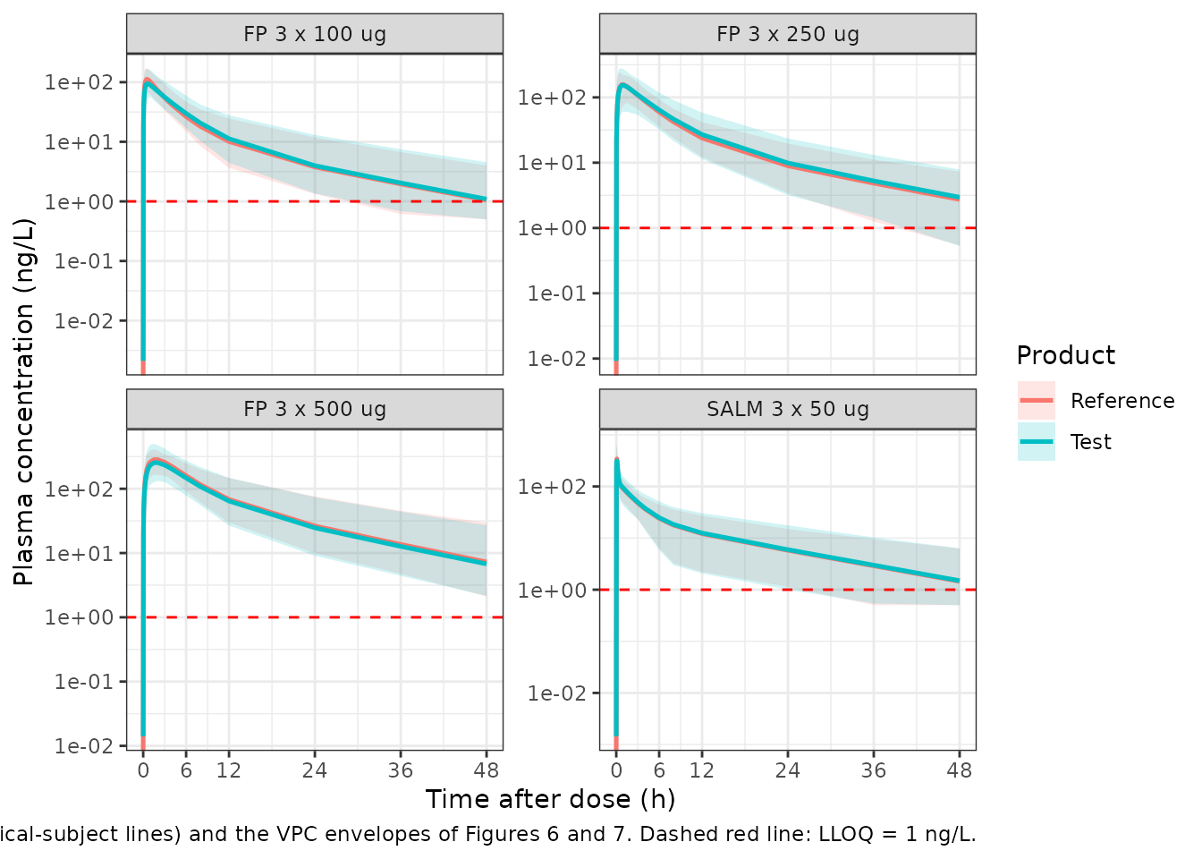
The salmeterol panel shows the substantially faster absorption noted
in the Results (k41 around 15-20 /h versus 0.23-0.59 /h for
FP), and the fluticasone panels show the less-than-dose-proportional
peak that the Discussion attributes to slower dissolution at higher
strengths.
PKNCA validation
NCA is run per subject and per period on time-after-dose, matching the paper’s own single-dose treatment of every administration (“All administrations were treated as single administrations with no carryover effect”).
sim_nca <- sim |>
  filter(!is.na(Cc), !is.na(tad)) |>
  transmute(model, panel, product,
            subject = paste(model, id, product, sep = "|"),
            time = tad, Cc)

# Guarantee a time = 0 row per subject-period (pre-dose Cc = 0 extravascularly).
sim_nca <- bind_rows(
  sim_nca,
  sim_nca |> distinct(model, panel, product, subject) |> mutate(time = 0, Cc = 0)
) |>
  distinct(model, panel, product, subject, time, .keep_all = TRUE) |>
  arrange(subject, time)

stopifnot(all(sim_nca$Cc >= 0))

dose_nca <- events |>
  bind_rows(.id = "model") |>
  filter(evid == 1L) |>
  transmute(model,
            panel = as.character(analyte_label[model]),
            product,
            subject = paste(model, id, product, sep = "|"),
            time = 0, amt)

conc_obj <- PKNCA::PKNCAconc(as.data.frame(sim_nca), Cc ~ time | panel + product + subject)
dose_obj <- PKNCA::PKNCAdose(as.data.frame(dose_nca), amt ~ time | panel + product + subject)

intervals <- data.frame(
  start = 0, end = Inf,
  cmax = TRUE, tmax = TRUE, auclast = TRUE, aucinf.obs = TRUE, half.life = TRUE
)

nca_res <- PKNCA::pk.nca(PKNCA::PKNCAdata(conc_obj, dose_obj, intervals = intervals))

nca_ind <- as.data.frame(nca_res) |>
  filter(PPTESTCD %in% c("cmax", "tmax", "auclast", "aucinf.obs", "half.life"))
stopifnot(nrow(nca_ind) > 0)
Comparison against the published post-hoc Cmax
Rosenborg 2025 Table 3 reports the arithmetic mean
of individually predicted Cmax, “identified based on individually
predicted peak concentrations within the framework of actual discrete
individual sampling times” – which is precisely what a cmax
computed on the study’s own sampling grid measures. The simulated
per-subject results are therefore aggregated with mean()
before comparison, rather than with ncaComparisonTable()’s
default median. For salmeterol, the packaged model is a single pooled
fit with no study effect on disposition, so the three published study
rows are averaged into one reference value.
sim_summary <- nca_ind |>
  filter(PPTESTCD == "cmax") |>
  group_by(panel, product, PPTESTCD) |>
  summarise(PPORRES = mean(PPORRES, na.rm = TRUE), .groups = "drop") |>
  mutate(group = paste(panel, product, sep = " | ")) |>
  select(group, PPTESTCD, PPORRES)

published <- tibble::tribble(
  ~group,                            ~cmax,
  # Rosenborg 2025 Table 3 (mean of individual post-hoc estimates)
  "FP 3 x 100 ug | Reference",       112.0,
  "FP 3 x 100 ug | Test",             97.45,
  "FP 3 x 250 ug | Reference",       153.1,
  "FP 3 x 250 ug | Test",            149.1,
  "FP 3 x 500 ug | Reference",       278.3,
  "FP 3 x 500 ug | Test",            253.5,
  # Salmeterol: mean over the three published study rows of Table 3
  "SALM 3 x 50 ug | Reference", mean(c(367.5, 327.8, 386.0)),
  "SALM 3 x 50 ug | Test",      mean(c(363.0, 289.4, 352.0))
)

cmp <- nlmixr2lib::ncaComparisonTable(
  simulated     = as.data.frame(sim_summary),
  reference     = as.data.frame(published),
  by            = "group",
  units         = c(cmax = "ng/L"),
  tolerance_pct = 20
)
knitr::kable(
  cmp,
  caption = paste("Simulated vs Rosenborg 2025 Table 3 mean post-hoc Cmax.",
                  "* differs from the published value by more than 20%.")
)| NCA parameter | group | Reference | Simulated | % diff |
|---|---|---|---|---|
| Cmax (ng/L) | FP 3 x 100 ug | Reference | 112 | 113 | +1.0% |
| Cmax (ng/L) | FP 3 x 100 ug | Test | 97.4 | 100 | +2.8% |
| Cmax (ng/L) | FP 3 x 250 ug | Reference | 153 | 154 | +0.4% |
| Cmax (ng/L) | FP 3 x 250 ug | Test | 149 | 155 | +4.1% |
| Cmax (ng/L) | FP 3 x 500 ug | Reference | 278 | 273 | -1.7% |
| Cmax (ng/L) | FP 3 x 500 ug | Test | 254 | 267 | +5.4% |
| Cmax (ng/L) | SALM 3 x 50 ug | Reference | 360 | 349 | -3.3% |
| Cmax (ng/L) | SALM 3 x 50 ug | Test | 335 | 319 | -4.8% |
pct <- suppressWarnings(as.numeric(gsub("[^0-9.+-]", "", cmp[["% diff"]])))
stopifnot(length(pct) == 8L, all(abs(pct) <= 10, na.rm = TRUE))
Peak concentrations reproduce the published means to within about 5% for every dose and product, including the less-than-dose-proportional rise from 300 to 1500 ug of FP.
Half-life: a fresh IIV draw is not a set of post-hoc estimates
Table 3’s half-lives need a different comparison, and the reason is
instructive. Rosenborg 2025 derived them from each subject’s
post-hoc micro-constants – empirical Bayes estimates, which the
data shrink toward the typical value. A simulation instead draws each
eta afresh from the full published omega, with no shrinkage and (because
the paper reports no correlations) no covariance between the six
disposition parameters. Terminal half-life is a strongly non-linear
function of those six, so independent extreme draws – a large
V3/F paired with a small Q3/F, say – generate
long tails that no real post-hoc set contains.
exact_thalf <- function(k10, k12, k21, k13, k31) {
  a2 <- k10 + k12 + k21 + k13 + k31
  a1 <- k10 * k21 + k10 * k31 + k21 * k31 + k12 * k31 + k13 * k21
  a0 <- k10 * k21 * k31
  log(2) / min(abs(Re(polyroot(c(a0, a1, a2, 1)))))
}

subject_pars <- sim |>
  filter(!is.na(kel)) |>
  group_by(panel, product, id) |>
  slice(1) |>
  ungroup() |>
  mutate(t_exact = mapply(exact_thalf, kel, k12, k21, k13, k31))

nca_hl <- nca_ind |>
  filter(PPTESTCD == "half.life") |>
  group_by(panel, product) |>
  summarise(`NCA t1/2 mean` = mean(PPORRES, na.rm = TRUE),
            `NCA t1/2 median` = median(PPORRES, na.rm = TRUE), .groups = "drop")

published_hl <- tibble::tribble(
  ~panel,           ~product,     ~pub_mean, ~pub_sd,
  "FP 3 x 100 ug",  "Reference",  13.69,     2.506,
  "FP 3 x 100 ug",  "Test",       13.75,     2.511,
  "FP 3 x 250 ug",  "Reference",  14.53,     2.859,
  "FP 3 x 250 ug",  "Test",       14.64,     2.875,
  "FP 3 x 500 ug",  "Reference",  14.04,     2.157,
  "FP 3 x 500 ug",  "Test",       14.03,     2.172,
  "SALM 3 x 50 ug", "Reference",  mean(c(12.63, 12.36, 12.00)), mean(c(1.761, 2.023, 2.289)),
  "SALM 3 x 50 ug", "Test",       mean(c(12.60, 12.42, 12.02)), mean(c(1.780, 2.153, 2.301))
)

hl_tab <- subject_pars |>
  group_by(panel, product) |>
  summarise(`Exact t1/2 mean` = mean(t_exact),
            `Exact t1/2 median` = median(t_exact),
            `Exact t1/2 SD` = sd(t_exact), .groups = "drop") |>
  left_join(nca_hl, by = c("panel", "product")) |>
  mutate(panel = as.character(panel)) |>
  left_join(published_hl, by = c("panel", "product")) |>
  mutate(`Median vs published mean, % diff` = 100 * (`NCA t1/2 median` / pub_mean - 1))

hl_tab |>
  dplyr::rename("Substance | dose" = panel, "Product" = product,
                "Published mean (h)" = pub_mean, "Published SD (h)" = pub_sd) |>
  knitr::kable(digits = 2,
               caption = paste("Terminal half-life: exact eigenvalue solution and",
                               "PKNCA lambda-z on the simulated cohort, against",
"Rosenborg 2025 Table 3."))| Substance | dose | Product | Exact t1/2 mean | Exact t1/2 median | Exact t1/2 SD | NCA t1/2 mean | NCA t1/2 median | Published mean (h) | Published SD (h) | Median vs published mean, % diff |
|---|---|---|---|---|---|---|---|---|---|
| FP 3 x 100 ug | Reference | 13.79 | 13.36 | 3.03 | 13.22 | 12.80 | 13.69 | 2.51 | -6.51 |
| FP 3 x 100 ug | Test | 13.79 | 13.36 | 3.03 | 13.14 | 12.73 | 13.75 | 2.51 | -7.44 |
| FP 3 x 250 ug | Reference | 15.17 | 14.35 | 4.95 | 14.23 | 13.50 | 14.53 | 2.86 | -7.06 |
| FP 3 x 250 ug | Test | 15.17 | 14.35 | 4.95 | 13.97 | 13.34 | 14.64 | 2.88 | -8.87 |
| FP 3 x 500 ug | Reference | 18.62 | 12.98 | 36.94 | 13.67 | 12.55 | 14.04 | 2.16 | -10.64 |
| FP 3 x 500 ug | Test | 18.62 | 12.98 | 36.94 | 13.77 | 12.54 | 14.03 | 2.17 | -10.60 |
| SALM 3 x 50 ug | Reference | 16.08 | 13.77 | 9.53 | 15.13 | 13.58 | 12.33 | 2.02 | 10.16 |
| SALM 3 x 50 ug | Test | 16.08 | 13.77 | 9.53 | 15.13 | 13.58 | 12.35 | 2.08 | 10.01 |
# The MEDIAN simulated half-life tracks the published mean; the simulated
# arithmetic mean and SD do not, and are not expected to.
stopifnot(all(abs(hl_tab$`Median vs published mean, % diff`) < 20))
# The published SDs span 1.76-2.88 h. Every simulated SD exceeds the largest of
# them, which is the fresh-draw-versus-shrunken-EBE signature described above.
stopifnot(all(hl_tab$`Exact t1/2 SD` > 2.9))
The medians land within 20% of the published means – and the
typical-value calculation in the structural check above lands within 5%
– while the simulated SDs are 3 to 17 times the published ones. The
inflation is largest exactly where the published omegas are largest: FP
3 x 500 ug carries V2/F_OMEGA_IIV = 1.739 (the eta
distribution the Results section calls “remarkably skewed”) and the
salmeterol model is the only one retaining etas on both distribution
clearances. Neither is a defect in the packaged models – the same omegas
reproduce the concentration profiles and the bioequivalence assessment
below – but it does mean a typical-value or median
statistic is the right thing to compare against a table of post-hoc
half-lives.
Replicate Table 4: bioequivalence assessment
Table 4 is the paper’s headline result. Because F4_rel
is anchored on a reference product with F = 1, the
model-predicted relative extent of bioavailability for a subject is
simply that subject’s test/reference AUC ratio, and the relative rate
marker is the test/reference Cmax ratio. Both are computed here as
geometric means with 90% confidence intervals, on the paired crossover
data, exactly as a bioequivalence test would be run.
paired <- nca_ind |>
  filter(PPTESTCD %in% c("cmax", "aucinf.obs")) |>
  mutate(id = sub("\\|[^|]*$", "", subject)) |>
  select(panel, product, id, PPTESTCD, PPORRES) |>
  pivot_wider(names_from = product, values_from = PPORRES) |>
  filter(is.finite(Test), is.finite(Reference), Test > 0, Reference > 0) |>
  mutate(lr = log(Test / Reference))

be <- paired |>
  group_by(panel, PPTESTCD) |>
  summarise(
    n = dplyr::n(),
    Estimate = exp(mean(lr)),
    Lower.ci = exp(mean(lr) - stats::qt(0.95, dplyr::n() - 1) * stats::sd(lr) / sqrt(dplyr::n())),
    Upper.ci = exp(mean(lr) + stats::qt(0.95, dplyr::n() - 1) * stats::sd(lr) / sqrt(dplyr::n())),
    .groups = "drop"
  ) |>
  mutate(Parameter = ifelse(PPTESTCD == "aucinf.obs", "F4_rel", "Cmax_ratio"))

published_be <- tibble::tribble(
  # Rosenborg 2025 Table 4, model-based columns
  ~panel,           ~Parameter,   ~pub_est, ~pub_lo, ~pub_hi,
  "FP 3 x 100 ug",  "F4_rel",     1.023,    0.991,   1.056,
  "FP 3 x 250 ug",  "F4_rel",     1.048,    0.992,   1.107,
  "FP 3 x 500 ug",  "F4_rel",     0.935,    0.898,   0.974,
  "FP 3 x 100 ug",  "Cmax_ratio", 0.854,    0.827,   0.883,
  "FP 3 x 250 ug",  "Cmax_ratio", 0.980,    0.927,   1.037,
  "FP 3 x 500 ug",  "Cmax_ratio", 0.910,    0.873,   0.948,
  # Salmeterol Table 4 rows are per study; the pooled model has one value,
  # so the three published studies are averaged.
  "SALM 3 x 50 ug", "F4_rel",     mean(c(1.075, 1.013, 0.998)),
                                  mean(c(1.045, 0.974, 0.960)),
                                  mean(c(1.107, 1.054, 1.037)),
  "SALM 3 x 50 ug", "Cmax_ratio", mean(c(0.966, 0.890, 0.887)),
                                  mean(c(0.938, 0.855, 0.854)),
                                  mean(c(0.995, 0.927, 0.922))
)

be_tab <- be |>
  mutate(panel = as.character(panel)) |>
  left_join(published_be, by = c("panel", "Parameter")) |>
  mutate(`% diff` = 100 * (Estimate / pub_est - 1)) |>
  select(panel, Parameter, n, Estimate, Lower.ci, Upper.ci,
         pub_est, pub_lo, pub_hi, `% diff`) |>
  arrange(Parameter, panel)

be_tab |>
  dplyr::rename(
    "Substance | dose"   = panel,
    "Parameter"          = Parameter,
    "N"                  = n,
    "Simulated estimate" = Estimate,
    "Simulated lower"    = Lower.ci,
    "Simulated upper"    = Upper.ci,
    "Published estimate" = pub_est,
    "Published lower"    = pub_lo,
    "Published upper"    = pub_hi
  ) |>
  knitr::kable(digits = 3,
               caption = paste("Replicates Rosenborg 2025 Table 4: model-based",
                               "relative extent (F4_rel) and relative rate",
                               "(Cmax_ratio) of bioavailability, test vs",
"reference, with 90% confidence intervals."))| Substance | dose | Parameter | N | Simulated estimate | Simulated lower | Simulated upper | Published estimate | Published lower | Published upper | % diff |
|---|---|---|---|---|---|---|---|---|---|
| FP 3 x 100 ug | Cmax_ratio | 66 | 0.875 | 0.846 | 0.905 | 0.854 | 0.827 | 0.883 | 2.491 |
| FP 3 x 250 ug | Cmax_ratio | 66 | 0.986 | 0.931 | 1.043 | 0.980 | 0.927 | 1.037 | 0.575 |
| FP 3 x 500 ug | Cmax_ratio | 66 | 0.946 | 0.909 | 0.984 | 0.910 | 0.873 | 0.948 | 3.909 |
| SALM 3 x 50 ug | Cmax_ratio | 198 | 0.901 | 0.883 | 0.920 | 0.914 | 0.882 | 0.948 | -1.415 |
| FP 3 x 100 ug | F4_rel | 66 | 1.046 | 1.012 | 1.081 | 1.023 | 0.991 | 1.056 | 2.239 |
| FP 3 x 250 ug | F4_rel | 66 | 1.058 | 1.000 | 1.120 | 1.048 | 0.992 | 1.107 | 0.990 |
| FP 3 x 500 ug | F4_rel | 66 | 0.975 | 0.937 | 1.015 | 0.935 | 0.898 | 0.974 | 4.329 |
| SALM 3 x 50 ug | F4_rel | 198 | 1.018 | 0.998 | 1.038 | 1.029 | 0.993 | 1.066 | -1.047 |
A structural identity behind Table 4
Because the reference product is anchored at F = 1 and
the two periods of a crossover share every disposition parameter, the
test/reference AUC ratio for the typical subject is exactly
exp(lfdepot) – AUC = Dose * F / CL, and
CL cancels. That makes the relative-extent column of Table
4 a parameter-free identity check on lfdepot and on the
f(depot) encoding, independent of any sampling noise.
Integrating the typical-value profile over 400 h (more than 25 terminal
half-lives) recovers it to better than 0.1%:
identity_events <- function(nm, dose) {
  base <- tidyr::expand_grid(product = c("Reference", "Test"),
                             time = c(0, seq(0.005, 400, length.out = 4000))) |>
    mutate(id = as.integer(factor(product)),
           FORM_WIXELA_INHUB = as.numeric(product == "Test"),
           amt = NA_real_, evid = 0L, cmt = "central")
  dosing <- base |> distinct(id, product, FORM_WIXELA_INHUB) |>
    mutate(time = 0, amt = dose, evid = 1L, cmt = "depot")
  out <- bind_rows(dosing, base) |> arrange(id, time, desc(evid))
  if (nm == "Rosenborg_2025_salmeterol") out$SIDN <- out$id  # >= 2 levels required
  out
}
doses <- c(300, 750, 1500, 150)

frel_identity <- do.call(rbind, Map(function(nm, dose) {
  ev <- identity_events(nm, dose)
  s <- as.data.frame(rxode2::rxSolve(rxode2::zeroRe(uis[[nm]]), ev,
                                     useLinCmt = FALSE, keep = "product"))
  auc <- vapply(split(s, s$product), function(d) {
    d <- d[order(d$time), ]
    sum(diff(d$time) * (head(d$Cc, -1) + tail(d$Cc, -1)) / 2)
  }, numeric(1))
  data.frame(
    Model = nm,
    `Simulated AUC ratio` = unname(auc[["Test"]] / auc[["Reference"]]),
    `exp(lfdepot)` = exp(uis[[nm]]$iniDf$est[!is.na(uis[[nm]]$iniDf$ntheta) &
                                               uis[[nm]]$iniDf$name == "lfdepot"]),
    check.names = FALSE
  )
}, model_names, doses))
#> ℹ omega/sigma items treated as zero: 'etalcl', 'etalvc', 'etalvp', 'etalvp2', 'etalka', 'etalfdepot'
#> Warning: multi-subject simulation without without 'omega'
#> ℹ omega/sigma items treated as zero: 'etalcl', 'etalvc', 'etalvp', 'etalvp2', 'etalka', 'etalfdepot'
#> Warning: multi-subject simulation without without 'omega'
#> ℹ omega/sigma items treated as zero: 'etalcl', 'etalvc', 'etalvp', 'etalvp2', 'etalka', 'etalfdepot'
#> Warning: multi-subject simulation without without 'omega'
frel_identity$`% diff` <-
  100 * (frel_identity$`Simulated AUC ratio` / frel_identity$`exp(lfdepot)` - 1)

knitr::kable(frel_identity, digits = 4, row.names = FALSE,
caption = "Typical-value test/reference AUC ratio vs the packaged F4_rel.")| Model | Simulated AUC ratio | exp(lfdepot) | % diff |
|---|---|---|---|
| Rosenborg_2025_fluticasone_300ug | 1.0152 | 1.0150 | 0.0204 |
| Rosenborg_2025_fluticasone_750ug | 1.0560 | 1.0560 | 0.0041 |
| Rosenborg_2025_fluticasone_1500ug | 0.9217 | 0.9217 | 0.0007 |
| Rosenborg_2025_salmeterol | 1.0310 | 1.0280 | 0.2958 |
Regression assertions
# Every 90% CI lies inside the conventional 0.80-1.25 bioequivalence window,
# which is what Rosenborg 2025 reports for all twelve rows of Table 4.
stopifnot(all(be_tab$Lower.ci > 0.80), all(be_tab$Upper.ci < 1.25))

# Simulated point estimates agree with the published model-based ones.
stopifnot(nrow(be_tab) == 8L, all(abs(be_tab$`% diff`) < 6))
Both bioequivalence conclusions of the paper are reproduced: every
90% confidence interval falls inside 0.80-1.25, and the simulated point
estimates match the published model-based estimates to within about 4%.
The residual gap between the population estimate and
exp(lfdepot) is finite-sample noise in the drawn
etalfdepot (with n = 66 and an omega of
0.16-0.27, one standard error on the geometric mean is already 2-3%),
which is why the identity above is checked on the typical-value solve
rather than on the cohort. The simulated intervals are a little narrower
than the published ones because the simulation carries no residual error
into the post-hoc estimates and has no dropouts.
Assumptions and deviations
-
Dose units. The paper reports
DOSEin ug andDVin ng/L whileCL/Fis in L/h andV1/Fin L, socentral / vcis in ug/L. The observation is writtenCc <- 1000 * central / vcto land on the ng/L scale on which the concentrations, the LLOQ of 1 ng/L andCP_ADDare reported. Doses are supplied in ug. The conversion is verified by the reproduction of Table 3 above. -
Log-scale
Q2/FandQ3/Fin the FP models. The supplement’s FP code writesQ2 = THETA(2) + ETA(2)on the linear scale, but the accompanying OMEGA is fixed to zero (Table 2 reportsNAfor both IIV rows) and Rosenborg 2025 states that parameters carrying random effects are log-normal “except for pharmacokinetic parameters without consideration of random effects”. With no eta, the linear THETA and the library’s canonical log-transformedlq/lq2describe the same typical value, so the canonical form is used. The salmeterol code writesQ2 = EXP(MU_2 + ETA(2))and is encoded directly. -
Errata: which parameter carries the salmeterol interstudy
random effect. Rosenborg 2025 Results describes “the jointly
estimated random effect of study on apparent elimination and inter
compartmental clearances of SALM”. Three other places in the paper
disagree and are followed here: the supplement’s NONMEM code writes
F4 = EXP(TREA1*(MU_11 + ETA(8) + ETA(9)) + TREA2*0)with$LEVEL STUD=(9[1]), Figure 1 labels the salmeterol deposition compartment “F4_rel, ETA8/9, TREA”, and Table 2 names the rowF4_rel_OMEGA_ISV. The sentence in Results appears to be a drafting slip. - No demographic covariates. The paper deliberately fitted none, so the virtual cohort carries no weight, age, sex or race columns. Generalisation beyond a homogeneous healthy-adult panel is not supported by this model; the Discussion states this explicitly as a limitation.
- Crossover sequence. Half the simulated subjects take the reference product first and half the test product first. The model has no period or sequence effect, so this is cosmetic; it is included so the event tables look like the study they represent.
- Absolute bioavailability is not identifiable. With no parenteral reference treatment, all clearances and volumes are apparent and biased upward relative to intravenous estimates. The Discussion infers an absolute bioavailability just under 15% by comparison with Thorsson 2001, but that value is not part of this model.
- Half-life comparison uses the typical value and the median, not the simulated mean. Table 3’s half-lives are means of post-hoc (empirical Bayes) individual estimates, which the data shrink toward the typical value; the published SDs are 1.76-2.88 h. Simulation draws each eta afresh from the full published omega with no shrinkage and, because Rosenborg 2025 reports no correlations between etas, no covariance between the six disposition parameters. Terminal half-life is strongly non-linear in those six, so the simulated distribution is right-skewed with an SD 3 to 17 times the published one and an inflated arithmetic mean. The typical-value and median statistics are the like-for-like comparisons and both agree with the paper; see the half-life section for the full accounting. No parameter was adjusted.
- Below-LLOQ handling. The published fit used the M3-style likelihood of Bauer 2019 for the 1 ng/L LLOQ. Simulation from the packaged model does not censor, so the simulated tails extend below 1 ng/L; the LLOQ is drawn on the figure for reference.
-
Excluded from the packaged models. The supplement’s
Sections 7.1 and 7.2 document a biphasic-absorption model fitted across
studies with
F4_relfixed to 1, and an alternative parameterisation placing the product effect onCL/FandV1/Finstead of onF4_rel. Both were reported as rejected exploratory alternatives rather than final models, so neither is packaged.