Upadacitinib ACR response Markov models (Mohamed 2019)
Source:vignettes/articles/Mohamed_2019_upadacitinib.Rmd
Mohamed_2019_upadacitinib.RmdModel and source
- Citation: Mohamed M-EF, Klunder B, Camp HS, Othman AA. Exposure-Response Analyses of Upadacitinib Efficacy in Phase II Trials in Rheumatoid Arthritis and Basis for Phase III Dose Selection. Clin Pharmacol Ther. 2019;106(6):1319-1327.
- Article: https://doi.org/10.1002/cpt.1543 (open access, PMC6896251). Parameter estimates are in Supporting Information Tables S1 and S2.
- Concentration driver: Klunder B, Mohamed M-EF, Othman AA. Clin
Pharmacokinet. 2018;57(8):977-988, https://doi.org/10.1007/s40262-017-0605-6, also packaged
on its own as
Klunder_2017_upadacitinib.
The paper fits two independent continuous-time Markov models, one per phase IIb trial, because the placebo response differed between the populations. Both are packaged:
| Model | Trial | Population |
|---|---|---|
Mohamed_2019_upadacitinib_tnfir |
BALANCE I | inadequate response to anti-TNF therapy |
Mohamed_2019_upadacitinib_mtxir |
BALANCE II | inadequate response to methotrexate |
mod_tnf <- readModelDb("Mohamed_2019_upadacitinib_tnfir")
mod_mtx <- readModelDb("Mohamed_2019_upadacitinib_mtxir")
ui_tnf <- rxode2::rxode2(mod_tnf)
#> ℹ parameter labels from comments will be replaced by 'label()'
ui_mtx <- rxode2::rxode2(mod_mtx)
#> ℹ parameter labels from comments will be replaced by 'label()'
Structure
Each patient occupies one of five states: no response, ACR20, ACR50, ACR70 or dropout (Figure 1 of the paper). Transitions are first-order, between adjacent response states and from any response state to the absorbing dropout state. Upadacitinib multiplies the three upward rates (K01, K12, K23) by
where Cp is the plasma concentration at that moment
(Methods equation; gamma = 1 in BALANCE II, which reports
no Hill factor). The packaged models carry the state-occupancy
probabilities as ODE states (s_noresp,
s_acr20, s_acr50, s_acr70,
s_dropout), so a solve returns the expected fraction of a
population in each state. The outputs prob_acr20,
prob_acr50 and prob_acr70 count patients at or
above each threshold who have not dropped out, which is the
non-responder-imputation (NRI) proportion the paper simulates.
The concentration comes from the Klunder 2017 population PK model,
rheumatoid arthritis arm, which the paper used to generate each
patient’s concentration-time profile (Methods, “Exposure-response
analyses methodology”). Model time is in hours to match that PK model;
the Markov rates are reported per day and are divided by 24 inside
model().
Population
BALANCE I (NCT01960855) randomised 276 patients with an inadequate response to anti-TNF biologics to placebo or immediate-release upadacitinib 3, 6, 12 or 18 mg twice daily for 12 weeks. BALANCE II (NCT02066389) randomised 300 biologic-naive patients with an inadequate response to methotrexate to placebo, 3, 6, 12 or 18 mg twice daily or 24 mg once daily; 298 were analysed. All patients stayed on background methotrexate. Both cohorts were about 80% female and mostly White (89% and 98%), with mean age 57 and 55 years, mean weight 78 and 75 kg, mean baseline DAS28-CRP 5.77 and 5.66, mean baseline hsCRP 13.4 and 13.3 mg/L, and 83-84% anti-CCP positive (Mohamed 2019 Table 1). ACR response was assessed at weeks 2, 4, 6, 8 and 12.
str(mod_tnf()$population)
#> List of 14
#>  $ species              : chr "human"
#>  $ n_subjects           : int 276
#>  $ n_studies            : int 1
#>  $ age_range            : chr "26-88 years (mean 57)"
#>  $ weight_range         : chr "42-134 kg (mean 78)"
#>  $ sex_female_pct       : num 80
#>  $ race_ethnicity       : Named num [1:4] 89 8 1 1
#>   ..- attr(*, "names")= chr [1:4] "White" "Black" "Asian" "Other"
#>  $ disease_state        : chr "Moderate-to-severe active rheumatoid arthritis with inadequate response to at least one anti-TNF biologic, on s"| __truncated__
#>  $ dose_range           : chr "Placebo or immediate-release upadacitinib 3, 6, 12 or 18 mg twice daily for 12 weeks"
#>  $ regions              : chr "Multinational"
#>  $ baseline_das28crp    : chr "5.77 +/- 0.92 (range 3.58-7.97)"
#>  $ baseline_crp         : chr "13.4 +/- 18.6 mg/L (range 0.08-135)"
#>  $ anti_ccp_positive_pct: num 83
#>  $ notes                : chr "Mohamed 2019 Table 1 (BALANCE I column). ACR visits at weeks 2, 4, 6, 8 and 12. Exposure-response fit in NONMEM"| __truncated__
str(mod_mtx()$population)
#> List of 14
#>  $ species              : chr "human"
#>  $ n_subjects           : int 298
#>  $ n_studies            : int 1
#>  $ age_range            : chr "19-82 years (mean 55)"
#>  $ weight_range         : chr "44-122 kg (mean 75)"
#>  $ sex_female_pct       : num 79
#>  $ race_ethnicity       : Named num [1:4] 98 1 0 1
#>   ..- attr(*, "names")= chr [1:4] "White" "Black" "Asian" "Other"
#>  $ disease_state        : chr "Moderate-to-severe active rheumatoid arthritis with inadequate response to methotrexate, biologic-naive, on sta"| __truncated__
#>  $ dose_range           : chr "Placebo or immediate-release upadacitinib 3, 6, 12 or 18 mg twice daily or 24 mg once daily for 12 weeks"
#>  $ regions              : chr "Multinational"
#>  $ baseline_das28crp    : chr "5.66 +/- 0.99 (range 3-8.25)"
#>  $ baseline_crp         : chr "13.3 +/- 18.2 mg/L"
#>  $ anti_ccp_positive_pct: num 84
#>  $ notes                : chr "Mohamed 2019 Table 1 (BALANCE II column). 300 patients enrolled, 298 analysed. ACR visits at weeks 2, 4, 6, 8 a"| __truncated__
Source trace
Every ini() value carries an in-file comment naming its
source. The table collects them.
| Parameter | BALANCE I (_tnfir) |
BALANCE II (_mtxir) |
Source |
|---|---|---|---|
llambda01 (K01) |
log(0.0209) /day | log(0.0132) /day (male) | Tables S1 / S2 |
llambda10 (K10) |
log(0.0339) /day | log(0.0550) /day (anti-CCP negative, DAS28-CRP 5.66) | Tables S1 / S2 |
llambda12 (K12) |
log(0.0309) /day | log(0.0204) /day | Tables S1 / S2 |
llambda21 (K21) |
log(0.0589) /day | log(0.0407) /day | Tables S1 / S2 |
llambda23 (K23) |
log(0.0269) /day | log(0.0234) /day | Tables S1 / S2 |
llambda32 (K32) |
log(0.0263) /day | log(0.0240) /day | Tables S1 / S2 |
llambda0d (K0D) |
log(0.00269) /day | log(0.00120) /day | Tables S1 / S2 |
llambda1d (K1D) |
log(0.000246) /day | log(0.000891) /day | Tables S1 / S2 |
llambda2d (K2D) |
log(0.000871) /day | log(0.000617) /day | Tables S1 / S2 |
llambda3d (K3D) |
fixed(log(1e-10)) /day | log(0.000468) /day | Table S1 (‘1E-10 (fixed)’) / Table S2 |
lemax |
log(0.766) | log(1.19) | Tables S1 / S2 |
lec50 |
log(12.2) ng/mL | log(2.97) ng/mL | Tables S1 / S2; text, Results |
lhill |
log(3.46) | (none; Hill = 1) | Table S1 ‘Hill factor’ |
e_early_emax (tvtshift) |
2.15 | (none) | Table S1 and footnote b: Emax x (1 + tvtshift) in the first two weeks |
e_crp_emax |
0.276 | (none) | Table S1 ‘Exponent for the Effect of Baseline hs-CRP on Emax’ |
e_das28_lambda10 |
(none) | -2.26 | Table S2 ‘Exponent for the Effect of Baseline DAS28-CRP on K10’ |
e_sexf_lambda01 |
(none) | 1.7 | Table S2 ‘Ratio of K01 in females relative to males’ |
e_anticcp_lambda10 |
(none) | 0.394 | Table S2 ‘Ratio of K10 in anti-CCP positive relative to negative status subject’ |
lka, lcl, lvc,
lvp, lq, ltlag
|
12.3 /h, 39.7 x 0.76 L/h, 146 L, 64.3 L, 3.23 L/h, 0.48 h | same | Klunder 2017 Table 3 (RA arm) |
e_sexf_cl, e_crcl_cl,
e_sexf_vc, e_wt_vc
|
log(0.86), 0.32, log(0.75), 0.50 | same | Klunder 2017 Table 3 |
etalka, etalcl, etalvc
|
2.25, 0.0676, 0.0729 | same | Klunder 2017 Table 3 (RA %ISV squared) |
| Upward-rate drug effect | 1 + emax * Cc^hill / (ec50^hill + Cc^hill) |
1 + emax * Cc / (ec50 + Cc) |
Methods equation; Figure 1 (drug acts on K01, K12, K23) |
| State ODEs | d/dt(s_*) |
same | Figure 1 schematic |
Model checks that need no cohort
Probability is conserved
The five state probabilities must sum to 1 at every time, with or without drug.
typical_subject <- data.frame(
  id = 1L, SEXF = 1, WT = 75, CRCL = 100, CRP = 13.4,
  SCORE_DAS28CRP = 5.66, ANTICCP_POS = 1
)

# One dosing record plus observation rows. Observation rows carry dvid = 1 so
# that rxode2 maps them to the first endpoint; every output column is returned
# on each row regardless.
make_events <- function(cov, dose, ii, obs_h) {
  n_dose <- round(84 * 24 / ii)
  dose_rows <- data.frame(
    id = cov$id, time = 0, amt = dose, evid = 1L, cmt = "depot",
    ii = ii, addl = n_dose - 1L, dvid = NA_integer_
  )
  obs_rows <- tidyr::expand_grid(id = cov$id, time = obs_h) |>
    mutate(amt = 0, evid = 0L, cmt = NA_character_, ii = 0, addl = 0L, dvid = 1L)
  bind_rows(dose_rows, obs_rows) |>
    left_join(cov, by = "id") |>
    arrange(id, time, desc(evid))
}

obs_week <- seq(0, 12) * 168
mb <- bind_rows(
  rxode2::rxSolve(rxode2::zeroRe(ui_tnf),
    events = make_events(typical_subject, 12, 12, obs_week),
    returnType = "data.frame"
  ) |> mutate(model = "BALANCE I"),
  rxode2::rxSolve(rxode2::zeroRe(ui_mtx),
    events = make_events(typical_subject, 12, 12, obs_week),
    returnType = "data.frame"
  ) |> mutate(model = "BALANCE II")
) |>
  mutate(total = s_noresp + s_acr20 + s_acr50 + s_acr70 + s_dropout)
#> ℹ omega/sigma items treated as zero: 'etalka', 'etalcl', 'etalvc'
#> ℹ omega/sigma items treated as zero: 'etalka', 'etalcl', 'etalvc'
stopifnot(max(abs(mb$total - 1)) < 1e-6)
range(mb$total)
#> [1] 1 1
Placebo arm against the matrix exponential
Without drug the chain is time-homogeneous, so the state
probabilities at time t are
p(0) %*% expm(Q t). The ODE solve must agree with that
closed form; both sides use the same rates, so the bound is tight.
markov_q <- function(k) {
  q <- matrix(0, 5, 5)
  q[1, 2] <- k[["k01"]]
  q[1, 5] <- k[["k0d"]]
  q[2, 1] <- k[["k10"]]
  q[2, 3] <- k[["k12"]]
  q[2, 5] <- k[["k1d"]]
  q[3, 2] <- k[["k21"]]
  q[3, 4] <- k[["k23"]]
  q[3, 5] <- k[["k2d"]]
  q[4, 3] <- k[["k32"]]
  q[4, 5] <- k[["k3d"]]
  diag(q) <- -rowSums(q)
  q
}
expm_eigen <- function(a) {
  e <- eigen(a)
  Re(e$vectors %*% diag(exp(e$values)) %*% solve(e$vectors))
}
k_tnf <- c(
  k01 = 0.0209, k10 = 0.0339, k12 = 0.0309, k21 = 0.0589, k23 = 0.0269,
  k32 = 0.0263, k0d = 0.00269, k1d = 0.000246, k2d = 0.000871, k3d = 1e-10
)
closed <- t(sapply(obs_week / 24, function(d) {
  as.vector(c(1, 0, 0, 0, 0) %*% expm_eigen(markov_q(k_tnf) * d))
}))
ode_pbo <- rxode2::rxSolve(rxode2::zeroRe(ui_tnf),
  events = make_events(typical_subject, 0, 12, obs_week),
  returnType = "data.frame"
)
#> ℹ omega/sigma items treated as zero: 'etalka', 'etalcl', 'etalvc'
ode_mat <- as.matrix(ode_pbo[, c("s_noresp", "s_acr20", "s_acr50", "s_acr70", "s_dropout")])
stopifnot(max(abs(ode_mat - closed)) < 1e-5)
max(abs(ode_mat - closed))
#> [1] 4.374119e-06
BALANCE I placebo against Figure 2
Placebo has no covariates in the BALANCE I model, so its trajectory is a single deterministic curve. Figure 2 (BALANCE I, placebo panel) plots the model median; the values below are read from it by eye (about 1 percentage point of reading error).
fig2_tnf_pbo <- tibble::tribble(
  ~week, ~acr20, ~acr50, ~acr70,
  2, 21, 5, 0,
  4, 31, 10, 2,
  6, 38, 13, 4,
  8, 41, 16, 4,
  12, 43, 16.5, 5
)
tnf_pbo <- ode_pbo |>
  mutate(week = time / 168) |>
  filter(week %in% fig2_tnf_pbo$week) |>
  transmute(
    week,
    sim_acr20 = 100 * prob_acr20, sim_acr50 = 100 * prob_acr50,
    sim_acr70 = 100 * prob_acr70
  ) |>
  left_join(fig2_tnf_pbo, by = "week")
knitr::kable(tnf_pbo, digits = 1, caption = "BALANCE I placebo, % responders (NRI): model vs Figure 2.")| week | sim_acr20 | sim_acr50 | sim_acr70 | acr20 | acr50 | acr70 |
|---|---|---|---|---|---|---|
| 2 | 20.5 | 3.4 | 0.4 | 21 | 5.0 | 0 |
| 4 | 30.9 | 8.2 | 1.8 | 31 | 10.0 | 2 |
| 6 | 36.6 | 12.2 | 3.7 | 38 | 13.0 | 4 |
| 8 | 39.9 | 15.2 | 5.4 | 41 | 16.0 | 4 |
| 12 | 43.0 | 19.0 | 8.2 | 43 | 16.5 | 5 |
stopifnot(
  max(abs(tnf_pbo$sim_acr20 - tnf_pbo$acr20)) < 3,
  max(abs(tnf_pbo$sim_acr50 - tnf_pbo$acr50)) < 4,
  max(abs(tnf_pbo$sim_acr70 - tnf_pbo$acr70)) < 4
)
The ACR20 curve tracks Figure 2 within two points at every visit. ACR50 and ACR70 at week 12 run about 3 points above the plotted median, which is the median of 100 simulated 56-patient trials rather than an expected proportion.
The text and Figure 3 give the BALANCE I placebo week-12 response as 34/12/3%, which the Table S1 rates do not reproduce (43/19/8%). The 34% equals the observed BALANCE I placebo ACR20 response by NRI reported in the trial publication (Kremer 2016, Arthritis Rheumatol 68:2867), so the placebo point in Figure 3 appears to be the observed rate rather than a model prediction. The packaged model keeps the Table S1 rates, which the paper’s own visual predictive check (Figure 2) agrees with.
BALANCE II placebo against the printed prediction
The BALANCE II placebo rates depend on sex, anti-CCP status and baseline DAS28-CRP, so the population placebo response is an average over the cohort. The expectation is computed deterministically on a covariate lattice: sex (79% female) x anti-CCP (84% positive) x 20 quantiles of a normal DAS28-CRP distribution (mean 5.66, SD 0.99, truncated to the observed 3-8.25), all from Table 1.
das_q <- pmin(pmax(qnorm((seq_len(20) - 0.5) / 20, 5.66, 0.99), 3), 8.25)
lattice <- tidyr::expand_grid(SEXF = c(0, 1), ANTICCP_POS = c(0, 1), SCORE_DAS28CRP = das_q) |>
  mutate(
    id = row_number(), WT = 75, CRCL = 100, CRP = 13.3,
    w = ifelse(SEXF == 1, 0.79, 0.21) * ifelse(ANTICCP_POS == 1, 0.84, 0.16) / 20
  )
mtx_pbo <- rxode2::rxSolve(rxode2::zeroRe(ui_mtx),
  events = make_events(lattice, 0, 12, 84 * 24),
  returnType = "data.frame"
) |>
  left_join(select(lattice, id, w), by = "id") |>
  summarise(
    acr20 = 100 * sum(w * prob_acr20), acr50 = 100 * sum(w * prob_acr50),
    acr70 = 100 * sum(w * prob_acr70)
  )
#> ℹ omega/sigma items treated as zero: 'etalka', 'etalcl', 'etalvc'
#> Warning: multi-subject simulation without without 'omega'
knitr::kable(
  bind_rows(
    mutate(mtx_pbo, source = "Model, BALANCE II lattice"),
    tibble(acr20 = 47, acr50 = 18, acr70 = 8, source = "Mohamed 2019 Results / Figure 3")
  ) |> relocate(source),
  digits = 1, caption = "BALANCE II placebo, week-12 % responders (NRI)."
)| source | acr20 | acr50 | acr70 |
|---|---|---|---|
| Model, BALANCE II lattice | 46.9 | 18.2 | 7.1 |
| Mohamed 2019 Results / Figure 3 | 47.0 | 18.0 | 8.0 |
The match also fixes the reference categories, which Table S2 does
not state. If women or anti-CCP-positive patients were the reference
instead of men and anti-CCP-negative patients, the same lattice gives a
week-12 ACR20 placebo response of 21-34% rather than 47%. Shifting an
indicator down by one (SEXF - 1,
ANTICCP_POS - 1) moves its reference level to the other
category, since the effects enter as ratio^indicator; the
placebo arm has no drug, so the PK use of SEXF does not
matter here.
alt_ref <- function(shift_sex, shift_anticcp) {
  ev <- make_events(lattice, 0, 12, 84 * 24) |>
    mutate(SEXF = SEXF - shift_sex, ANTICCP_POS = ANTICCP_POS - shift_anticcp)
  rxode2::rxSolve(rxode2::zeroRe(ui_mtx), events = ev, returnType = "data.frame") |>
    left_join(select(lattice, id, w), by = "id") |>
    summarise(
      female_reference = shift_sex == 1, anticcp_positive_reference = shift_anticcp == 1,
      acr20 = 100 * sum(w * prob_acr20)
    )
}
alt <- bind_rows(alt_ref(1, 0), alt_ref(0, 1), alt_ref(1, 1))
#> ℹ omega/sigma items treated as zero: 'etalka', 'etalcl', 'etalvc'
#> Warning: multi-subject simulation without without 'omega'
#> ℹ omega/sigma items treated as zero: 'etalka', 'etalcl', 'etalvc'
#> Warning: multi-subject simulation without without 'omega'
#> ℹ omega/sigma items treated as zero: 'etalka', 'etalcl', 'etalvc'
#> Warning: multi-subject simulation without without 'omega'
knitr::kable(alt, digits = 1, caption = "BALANCE II placebo week-12 ACR20 under the other reference readings.")| female_reference | anticcp_positive_reference | acr20 |
|---|---|---|
| TRUE | FALSE | 33.7 |
| FALSE | TRUE | 30.4 |
| TRUE | TRUE | 20.6 |
Virtual cohorts
Each trial is simulated with 200 patients per arm and the arms of that trial. Covariates are drawn from the Table 1 summaries. Creatinine clearance is not reported in the paper and is drawn log-normally around 100 mL/min with a 30% coefficient of variation. Baseline hsCRP is right-skewed (mean 13.4, SD 18.6 mg/L), so it is drawn from the log-normal distribution with that mean and SD.
# rxode2 draws the PK random effects from its own stream, which is partitioned
# per solver thread, so the cohort differs between machines. Every assertion
# below is a centre or tolerance check that holds for any cohort.
set.seed(20190603)
n_per_arm <- 200L

draw_cohort <- function(trial, arm, n, id_offset) {
  is_tnf <- trial == "BALANCE I"
  crp_sdlog <- sqrt(log(1 + (18.6 / 13.4)^2))
  tibble(
    id = id_offset + seq_len(n),
    trial = trial,
    arm = arm,
    SEXF = rbinom(n, 1, if (is_tnf) 0.80 else 0.79),
    WT = if (is_tnf) {
      pmin(pmax(rnorm(n, 78, 17), 42), 134)
    } else {
      pmin(pmax(rnorm(n, 75, 14), 44), 122)
    },
    CRCL = exp(rnorm(n, log(100), 0.3)),
    CRP = pmin(pmax(exp(rnorm(n, log(13.4) - crp_sdlog^2 / 2, crp_sdlog)), 0.08), 135),
    SCORE_DAS28CRP = pmin(pmax(rnorm(n, 5.66, 0.99), 3), 8.25),
    ANTICCP_POS = rbinom(n, 1, 0.84)
  )
}

arms <- tibble::tribble(
  ~trial, ~arm, ~dose, ~ii,
  "BALANCE I", "Placebo", 0, 12,
  "BALANCE I", "3 mg BID", 3, 12,
  "BALANCE I", "6 mg BID", 6, 12,
  "BALANCE I", "12 mg BID", 12, 12,
  "BALANCE I", "18 mg BID", 18, 12,
  "BALANCE II", "Placebo", 0, 12,
  "BALANCE II", "3 mg BID", 3, 12,
  "BALANCE II", "6 mg BID", 6, 12,
  "BALANCE II", "12 mg BID", 12, 12,
  "BALANCE II", "18 mg BID", 18, 12,
  "BALANCE II", "24 mg QD", 24, 24
) |>
  mutate(arm_index = row_number())

# ACR visits plus a dense grid over the last dosing interval for the NCA.
obs_h <- sort(unique(c(seq(0, 12) * 168, seq(83 * 24, 84 * 24, by = 0.5))))

events <- bind_rows(lapply(seq_len(nrow(arms)), function(i) {
  cov <- draw_cohort(arms$trial[i], arms$arm[i], n_per_arm, (i - 1L) * n_per_arm)
  make_events(cov, arms$dose[i], arms$ii[i], obs_h)
}))
sim_trial <- function(ui, trial_name) {
  ev <- filter(events, trial == trial_name)
  sim <- rxode2::rxSolve(ui, events = ev, keep = c("trial", "arm"), returnType = "data.frame")
  stopifnot(length(unique(sim$id)) == length(unique(ev$id)))
  sim
}
sim <- bind_rows(
  sim_trial(ui_tnf, "BALANCE I"),
  sim_trial(ui_mtx, "BALANCE II")
) |>
  mutate(arm = factor(arm, levels = unique(arms$arm)))
Replicating Figure 2: ACR response time course
The lines are the expected proportion of responders (mean of the per-patient state probabilities) in each simulated arm.
fig2 <- sim |>
  filter(time %in% (seq(0, 12) * 168)) |>
  group_by(trial, arm, week = time / 168) |>
  summarise(
    ACR20 = 100 * mean(prob_acr20), ACR50 = 100 * mean(prob_acr50),
    ACR70 = 100 * mean(prob_acr70), .groups = "drop"
  ) |>
  pivot_longer(c(ACR20, ACR50, ACR70), names_to = "endpoint", values_to = "pct")

ggplot(fig2, aes(week, pct, colour = endpoint)) +
  geom_line(linewidth = 0.8) +
  facet_grid(trial ~ arm) +
  scale_x_continuous(breaks = c(0, 4, 8, 12)) +
  labs(
    x = "Time (weeks)", y = "% of patients (NRI)", colour = NULL,
    caption = "Replicates Figure 2 of Mohamed 2019 (model lines only)."
  ) +
  theme_bw() +
  theme(legend.position = "bottom")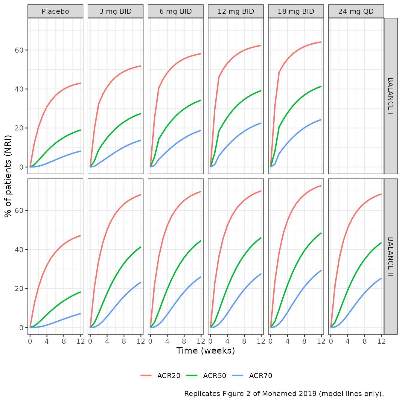
Replicating Figure 3: week-12 response by dose
Figure 3 plots the simulated week-12 NRI response for each twice-daily immediate-release dose. The reference values below are read from it by eye (about 1-2 percentage points of reading error).
fig3_ref <- tibble::tribble(
  ~trial, ~dose, ~acr20, ~acr50, ~acr70,
  "BALANCE I", 3, 53, 30, 16,
  "BALANCE I", 6, 57, 35, 20,
  "BALANCE I", 12, 62, 40, 24,
  "BALANCE I", 18, 63, 41, 25,
  "BALANCE II", 0, 47, 18, 8,
  "BALANCE II", 3, 67, 40, 22,
  "BALANCE II", 6, 69, 43, 25,
  "BALANCE II", 12, 71, 46, 28,
  "BALANCE II", 18, 72, 47, 29
)

wk12 <- sim |>
  filter(time == 84 * 24) |>
  left_join(select(arms, trial, arm, dose, ii), by = c("trial", "arm")) |>
  group_by(trial, arm, dose, ii) |>
  summarise(
    acr20 = 100 * mean(prob_acr20), acr50 = 100 * mean(prob_acr50),
    acr70 = 100 * mean(prob_acr70), .groups = "drop"
  )

fig3_cmp <- wk12 |>
  filter(ii == 12) |>
  inner_join(fig3_ref, by = c("trial", "dose"), suffix = c("_sim", "_fig3"))
fig3_cmp |>
  arrange(trial, dose) |>
  select(trial, arm, acr20_sim, acr20_fig3, acr50_sim, acr50_fig3, acr70_sim, acr70_fig3) |>
  dplyr::rename(
    Trial = trial, Arm = arm,
    "ACR20 sim" = acr20_sim, "ACR20 Fig 3" = acr20_fig3,
    "ACR50 sim" = acr50_sim, "ACR50 Fig 3" = acr50_fig3,
    "ACR70 sim" = acr70_sim, "ACR70 Fig 3" = acr70_fig3
  ) |>
knitr::kable(digits = 1, caption = "Week-12 % responders (NRI): simulation vs Figure 3.")| Trial | Arm | ACR20 sim | ACR20 Fig 3 | ACR50 sim | ACR50 Fig 3 | ACR70 sim | ACR70 Fig 3 |
|---|---|---|---|---|---|---|---|
| BALANCE I | 3 mg BID | 51.8 | 53 | 27.4 | 30 | 13.7 | 16 |
| BALANCE I | 6 mg BID | 58.1 | 57 | 34.3 | 35 | 18.8 | 20 |
| BALANCE I | 12 mg BID | 62.3 | 62 | 39.2 | 40 | 22.5 | 24 |
| BALANCE I | 18 mg BID | 64.1 | 63 | 41.4 | 41 | 24.4 | 25 |
| BALANCE II | Placebo | 47.2 | 47 | 18.3 | 18 | 7.2 | 8 |
| BALANCE II | 3 mg BID | 68.1 | 67 | 41.4 | 40 | 23.2 | 22 |
| BALANCE II | 6 mg BID | 69.8 | 69 | 44.6 | 43 | 26.1 | 25 |
| BALANCE II | 12 mg BID | 70.1 | 71 | 46.1 | 46 | 27.6 | 28 |
| BALANCE II | 18 mg BID | 72.8 | 72 | 48.6 | 47 | 29.4 | 29 |
stopifnot(
  nrow(fig3_cmp) == nrow(fig3_ref),
  max(abs(fig3_cmp$acr20_sim - fig3_cmp$acr20_fig3)) < 5,
  max(abs(fig3_cmp$acr50_sim - fig3_cmp$acr50_fig3)) < 5,
  max(abs(fig3_cmp$acr70_sim - fig3_cmp$acr70_fig3)) < 5
)
wk12 |>
  filter(ii == 12) |>
  pivot_longer(c(acr20, acr50, acr70), names_to = "endpoint", values_to = "pct") |>
  ggplot(aes(dose, pct, colour = endpoint)) +
  geom_line() +
  geom_point() +
  geom_point(
    data = pivot_longer(fig3_ref, c(acr20, acr50, acr70), names_to = "endpoint", values_to = "pct"),
    shape = 4, size = 3
  ) +
  facet_wrap(~trial) +
  labs(
    x = "Upadacitinib immediate-release dose, twice daily (mg)",
    y = "% of patients at week 12 (NRI)", colour = NULL,
    caption = "Lines: simulation. Crosses: Figure 3 of Mohamed 2019 (read by eye)."
  ) +
  theme_bw()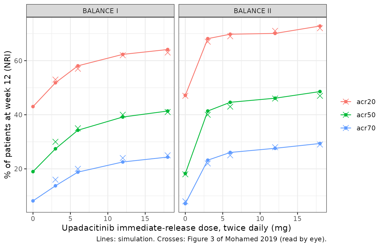
Both trials reproduce Figure 3 within a few percentage points at every dose. The BALANCE I placebo point of Figure 3 (34/12/3%) is left out of the comparison for the reason given above.
Choice of the hsCRP centring value
Table S1 gives the exponent of baseline hsCRP on Emax (0.276) but not
the value it is normalised to. The BALANCE I model uses 13.4 mg/L, the
baseline mean in Table 1. Because the effect is a power of
CRP / 13.4, a different reference r is
equivalent to rescaling the CRP column by 13.4 / r. The
table below shows the week-12 response of the 12 mg twice-daily arm
under three readings. The mean matches Figure 3 (62/40/24%) most
closely, the log-normal median overshoots by about 3 points, and an
uncentred effect overshoots by more than 10.
crp_ref_check <- function(ref) {
  ev <- filter(events, trial == "BALANCE I", arm == "12 mg BID", time %in% c(0, 84 * 24)) |>
    mutate(CRP = CRP * 13.4 / ref)
  rxode2::rxSolve(ui_tnf, events = ev, returnType = "data.frame") |>
    filter(time == 84 * 24) |>
    summarise(
      reference = ref, acr20 = 100 * mean(prob_acr20),
      acr50 = 100 * mean(prob_acr50), acr70 = 100 * mean(prob_acr70)
    )
}
crp_tab <- bind_rows(lapply(c(13.4, 7.8, 1), crp_ref_check))
knitr::kable(
  crp_tab |> dplyr::rename("hsCRP reference (mg/L)" = reference),
  digits = 1,
  caption = "BALANCE I, 12 mg BID, week 12: effect of the hsCRP centring value (7.8 mg/L is the median implied by a log-normal with the Table 1 mean and SD; 1 mg/L is no centring)."
)| hsCRP reference (mg/L) | acr20 | acr50 | acr70 |
|---|---|---|---|
| 13.4 | 62.9 | 39.9 | 23.2 |
| 7.8 | 65.0 | 42.5 | 25.3 |
| 1.0 | 76.0 | 57.3 | 38.5 |
stopifnot(crp_tab$acr20[crp_tab$reference == 1] - 62 > 8)PKNCA: steady-state average concentration
Table 2 of the paper lists the model-estimated average concentration over a dosing interval (Cave) at steady state for each arm. Cave is computed with PKNCA over the last dosing interval of the 12-week simulation.
conc <- sim |>
  filter(arm != "Placebo", time >= 83 * 24, !is.na(Cc)) |>
  left_join(select(arms, trial, arm, ii), by = c("trial", "arm")) |>
  mutate(treatment = paste(trial, arm, sep = ": "), tad = time - (84 * 24 - ii)) |>
  filter(tad >= 0) |>
  select(id, treatment, ii, tad, Cc)

conc_obj <- PKNCA::PKNCAconc(conc, Cc ~ tad | treatment + id)
intervals <- conc |>
  distinct(treatment, ii) |>
  transmute(treatment, start = 0, end = ii, cav = TRUE)
nca_res <- PKNCA::pk.nca(PKNCA::PKNCAdata(conc_obj, intervals = intervals))
#> No dose information provided, calculations requiring dose will return NA.

table2 <- tibble::tribble(
  ~treatment, ~cav,
  "BALANCE I: 3 mg BID", 9.2,
  "BALANCE I: 6 mg BID", 18.4,
  "BALANCE I: 12 mg BID", 39,
  "BALANCE I: 18 mg BID", 51.2,
  "BALANCE II: 3 mg BID", 9.7,
  "BALANCE II: 6 mg BID", 19.7,
  "BALANCE II: 12 mg BID", 40.5,
  "BALANCE II: 18 mg BID", 59.8,
  "BALANCE II: 24 mg QD", 35.9
)
cmp <- nlmixr2lib::ncaComparisonTable(
  simulated = nca_res,
  reference = table2,
  by = "treatment",
  units = c(cav = "ng/mL"),
  tolerance_pct = 20
)
knitr::kable(cmp, caption = "Median steady-state Cave: simulation vs Table 2. * differs by >20%.")| NCA parameter | treatment | Reference | Simulated | % diff |
|---|---|---|---|---|
| Cavg (ng/mL) | BALANCE I: 3 mg BID | 9.2 | 9.6 | +4.4% |
| Cavg (ng/mL) | BALANCE I: 6 mg BID | 18.4 | 18.9 | +2.8% |
| Cavg (ng/mL) | BALANCE I: 12 mg BID | 39 | 38.4 | -1.6% |
| Cavg (ng/mL) | BALANCE I: 18 mg BID | 51.2 | 56.2 | +9.8% |
| Cavg (ng/mL) | BALANCE II: 3 mg BID | 9.7 | 9.21 | -5.0% |
| Cavg (ng/mL) | BALANCE II: 6 mg BID | 19.7 | 19 | -3.7% |
| Cavg (ng/mL) | BALANCE II: 12 mg BID | 40.5 | 36.9 | -8.8% |
| Cavg (ng/mL) | BALANCE II: 18 mg BID | 59.8 | 60.9 | +1.8% |
| Cavg (ng/mL) | BALANCE II: 24 mg QD | 35.9 | 36 | +0.3% |
cav_sim <- as.data.frame(nca_res$result) |>
  filter(PPTESTCD == "cav") |>
  group_by(treatment) |>
  summarise(cav_sim = median(PPORRES), .groups = "drop") |>
  inner_join(table2, by = "treatment")
stopifnot(
  nrow(cav_sim) == nrow(table2),
  abs(median(100 * (cav_sim$cav_sim / cav_sim$cav - 1))) < 10,
  max(abs(100 * (cav_sim$cav_sim / cav_sim$cav - 1))) < 20
)
The Klunder 2017 PK model reproduces the Table 2 medians within about 10%, confirming that the packaged concentration driver is the one the paper used.
Assumptions and deviations
- Concentration driver. The paper drove the Markov models with each patient’s post hoc Klunder 2017 PK profile. The packaged models embed the Klunder 2017 rheumatoid-arthritis PK model with its between-subject variability, so simulated patients have population-sampled rather than individually estimated profiles. The PK residual error is not carried because the exposure-response fit used predicted, not observed, concentrations.
- No random effects in the Markov part. Tables S1 and S2 report no between-subject variability on the transition rates, so none is encoded.
- hsCRP centring (BALANCE I). Not printed; 13.4 mg/L (the Table 1 mean) is used. Of the readings tested it matches Figure 3 most closely (see above).
- DAS28-CRP centring (BALANCE II). Not printed; 5.66 (the Table 1 mean) is used. With this value the cohort placebo response reproduces the printed 47/18/8%.
- Reference categories (BALANCE II). Men and anti-CCP-negative patients are the reference, as the row labels of Table S2 imply. The placebo prediction confirms it (see above).
- Early Emax window (BALANCE I). Emax is multiplied by (1 + tvtshift) for the first 336 h (two weeks) after the first dose, assumed to be at time 0.
- BALANCE I placebo prediction in the text. The 34/12/3% quoted in the Results and plotted in Figure 3 is not reproduced (the Table S1 rates give 43/19/8%); the Table S1 rates agree with Figure 2, and the 34% equals the observed placebo ACR20 response in BALANCE I.
-
Extended-release regimens. The paper’s headline
simulations of 15 and 30 mg once-daily extended-release upadacitinib use
absorption parameters for the extended-release tablet estimated in a
separate phase I analysis (Mohamed 2019, Clin Pharmacol Drug
Dev 8:208), which this paper does not print. They are not
reproduced here. The packaged models accept any dosing into
depot, so an extended-release absorption model can be substituted by editing the PK block. -
Placeholder residual error. The Markov likelihood
is categorical, so the
prob_acr*outputs carry a fixed additive residual SD of 0.001 only so that nlmixr2 accepts the model. - Creatinine clearance. Not reported in the paper; drawn around 100 mL/min for the virtual cohorts. It affects only the PK driver.
-
Naming. The paper’s K01 … K3D are named
lambda01…lambda3dbecausek12/k21are the PK micro-constants in the same model. Baseline anti-CCP status uses theANTICCP_POScovariate column. The state-occupancy compartments follow thes_<state>shape of the other multistate models in the library (Lin_2024_TB_multistate,Ibrahim_2023_ibrutinib_competing_risk); the register has no canonical entry for them, socheckModelConventions()reports one non-canonical compartment warning per state.