Nicotinic acid / NEFA (Ahlstrom 2010) -- rat
Source:vignettes/articles/Ahlstrom_2010_nicotinicAcid_rat.Rmd
Ahlstrom_2010_nicotinicAcid_rat.RmdModel and source
- Citation: Ahlstrom C, Peletier LA, Jansson-Lofmark R, Gabrielsson J. Feedback modeling of non-esterified fatty acids in rats after nicotinic acid infusions. J Pharmacokinet Pharmacodyn 2011;38(1):1-24.
- Article (open access): doi:10.1007/s10928-010-9172-2
Population
The model was developed from 63 male Sprague-Dawley rats (Harlan Nederlands B.V.; body weight 220-367 g) studied at AstraZeneca R&D Molndal, Sweden. Rats were instrumented with arterial (carotid) and venous (jugular) catheters and allowed 5-8 days of recovery. They were fasted 14 h prior to dosing and throughout the experiment.
Animals received an IV constant-rate infusion of nicotinic acid (NiAc) or vehicle in 8 groups: vehicle / 1 / 5 / 20 umol/kg over 30 min (n = 10 / 4 / 8 / 9) and vehicle / 5 / 10 / 51 umol/kg over 300 min (n = 8 / 9 / 8 / 7). NiAc was measured by LC-MS (LLOQ 1 nmol/L, linear 0.001-28 umol/L) and NEFA by enzymatic colorimetric assay.
Endogenous NiAc was estimated to be 6.8 nmol/L on average (population range 4.8-15 nmol/L per Eq. 12 / Appendix A); baseline NEFA ranged 0.3-1.1 mmol/L.
The same information is available programmatically via the model’s
population metadata
(readModelDb("Ahlstrom_2010_nicotinicAcid_rat")$population).
Source trace
Per-parameter origin is recorded as an in-file comment next to each
ini() entry in
inst/modeldb/specificDrugs/Ahlstrom_2010_nicotinicAcid_rat.R.
The table below collects them in one place for review.
| Equation / parameter | Value | Source location |
|---|---|---|
Vmax1 (lvmax_hi) |
0.0573 umol/min/kg (RSE 1.57%) | Table 1 |
Km1 (lkm_hi) |
0.00468 umol/L (RSE 1.97%) | Table 1 |
Vmax2 (lvmax_lo) |
1.46 umol/min/kg (RSE 4.20%) | Table 1 |
Km2 (lkm_lo) |
16.6 umol/L (RSE 6.20%) | Table 1 |
Vc (lvc) |
0.345 L/kg (RSE 0.559%) | Table 1 |
Cld -> Q (lq) |
0.0203 L/min/kg (RSE 3.08%) | Table 1 |
Vt -> Vp (lvp) |
3.54 L/kg (RSE 7.66%) | Table 1 |
Synt (lsynt) |
0.0346 umol/min/kg (RSE 4.10%) | Table 1 |
R0 (lr0) |
0.606 mmol/L (RSE 3.51%) | Table 2 |
kout (lkout) |
0.411 L/mmol/min (RSE 9.22%) | Table 2 |
ktol (lktol) |
0.0267 1/min (RSE 3.40%) | Table 2 |
IC50 (lic50) |
0.0446 umol/L (RSE 7.20%) | Table 2 |
gamma (lgam) |
1.48 (RSE 3.79%) | Table 2 |
p (lpmod) |
1.21 (RSE 6.64%) | Table 2 |
kcap (lkcap) |
0.0318 mmol/L/min (RSE 6.51%) | Table 2 |
| Imax | 1 (fixed) | Table 2 + Discussion |
| IIV Vmax2 (CV) | 98.2% (RSE 24.8) | Table 1 |
| IIV Cld (CV) | 54.5% (RSE 88.6) | Table 1 |
| IIV Synt (CV) | 15.8% (RSE 62.5) | Table 1 |
| IIV R0 (CV) | 29.0% (RSE 43.1) | Table 2 |
| IIV kout (CV) | 48.2% (RSE 35.6) | Table 2 |
| IIV IC50 (CV) | 101% (RSE 46.1) | Table 2 |
| r1 prop. (NiAc) | 34.4% (RSE 18.6) | Table 1 |
| r2 add. (NiAc) | 0.800 (RSE 5.80) | Table 1 – see Assumptions |
| r prop. (NEFA) | 22.1% (RSE 8.51) | Table 2 |
| NiAc disposition ODEs | n/a | Eqs. 1a-1b + Fig. 1 |
| Drug inhibition I(Cp) | n/a | Eq. 2 |
| NEFA balance ODE | n/a | Eq. 3 |
| Moderator chain (N=8) | n/a | Eq. 4 + Results “optimal N was 8” |
| kin steady-state form | kin = R0^p * (kout * R0^2 - kcap) | Text following Eq. 4 |
| Endogenous Cp baseline | quadratic root (Cp_0 ~ 6.8 nmol/L) | Appendix A Eqs. 9-12 |
Loading the model
mod <- readModelDb("Ahlstrom_2010_nicotinicAcid_rat")
mod_typical <- rxode2::zeroRe(mod)
#> ℹ parameter labels from comments will be replaced by 'label()'
Helper to build an event table with one IV infusion plus matched
observation rows on the Cc (NiAc) and NEFA
outputs:
make_events <- function(dose_umolkg, dur_min, tmax = 600, dt = 1, id_offset = 0L) {
  times <- seq(-30, tmax, by = dt)
  obs_Cc   <- data.frame(id = id_offset + 1L, time = times,
                         evid = 0, amt = 0, rate = NA_real_, cmt = "Cc")
  obs_NEFA <- data.frame(id = id_offset + 1L, time = times,
                         evid = 0, amt = 0, rate = NA_real_, cmt = "NEFA")
  if (dose_umolkg > 0) {
    dose <- data.frame(
      id   = id_offset + 1L,
      time = 0,
      evid = 1,
      amt  = dose_umolkg,
      rate = dose_umolkg / dur_min,
      cmt  = "central"
    )
    dplyr::bind_rows(dose, obs_Cc, obs_NEFA)
  } else {
    dplyr::bind_rows(obs_Cc, obs_NEFA)
  }
}
Replicating published figures (typical-value)
We replicate the typical-value behaviour of two dose scenarios studied in the paper:
- a short, high infusion (20 umol/kg over 30 min) showing rapid Cp excursion, near-complete NEFA suppression, and limited tolerance;
- a long infusion (51 umol/kg over 300 min) showing tolerance development (NEFA recovery during continued infusion) followed by a clear rebound above baseline after infusion cessation.
ev_30 <- make_events(dose_umolkg = 20, dur_min = 30, tmax = 200)
sim_30 <- as.data.frame(rxSolve(mod_typical, ev_30))
#> ℹ omega/sigma items treated as zero: 'etalvmax_lo', 'etalq', 'etalsynt', 'etalrbase', 'etalkout', 'etalic50'
#> Warning:
#> with negative times, compartments initialize at first negative observed time
#> with positive times, compartments initialize at time zero
#> use 'rxSetIni0(FALSE)' to initialize at first observed time
#> this warning is displayed once per session

ggplot(sim_30, aes(time, Cc)) +
  geom_line(linewidth = 0.7) +
  geom_vline(xintercept = c(0, 30), linetype = "dashed", colour = "grey50") +
  labs(x = "Time (min)", y = "NiAc Cp (umol/L)",
       title = "NiAc plasma concentration -- 20 umol/kg / 30 min infusion",
       caption = "Replicates Fig. 2a (high-dose 30-min infusion) of Ahlstrom 2010, typical-value.")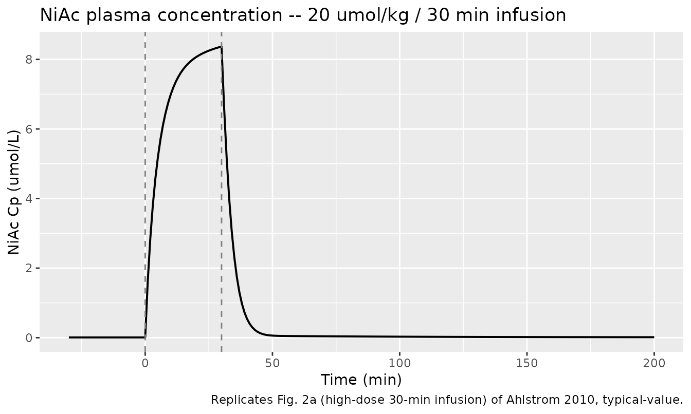
ggplot(sim_30, aes(time, NEFA)) +
  geom_line(linewidth = 0.7) +
  geom_hline(yintercept = 0.606, linetype = "dotted", colour = "grey50") +
  geom_vline(xintercept = c(0, 30), linetype = "dashed", colour = "grey50") +
  labs(x = "Time (min)", y = "NEFA (mmol/L)",
       title = "NEFA response -- 20 umol/kg / 30 min infusion",
       caption = "Replicates Fig. 6a (NEFA after 30-min infusion) of Ahlstrom 2010, typical-value.")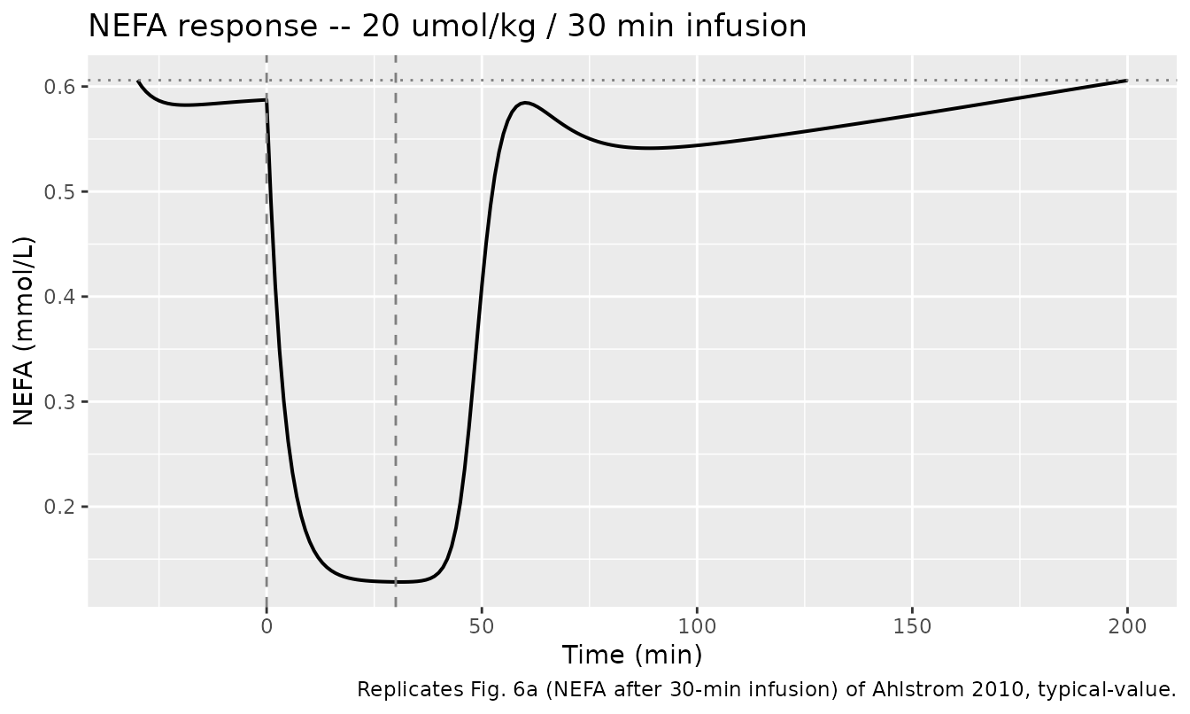
ev_300 <- make_events(dose_umolkg = 51, dur_min = 300, tmax = 600)
sim_300 <- as.data.frame(rxSolve(mod_typical, ev_300))
#> ℹ omega/sigma items treated as zero: 'etalvmax_lo', 'etalq', 'etalsynt', 'etalrbase', 'etalkout', 'etalic50'

ggplot(sim_300, aes(time, Cc)) +
  geom_line(linewidth = 0.7) +
  geom_vline(xintercept = c(0, 300), linetype = "dashed", colour = "grey50") +
  labs(x = "Time (min)", y = "NiAc Cp (umol/L)",
       title = "NiAc plasma concentration -- 51 umol/kg / 300 min infusion",
       caption = "Replicates Fig. 2b (high-dose 300-min infusion) of Ahlstrom 2010, typical-value.")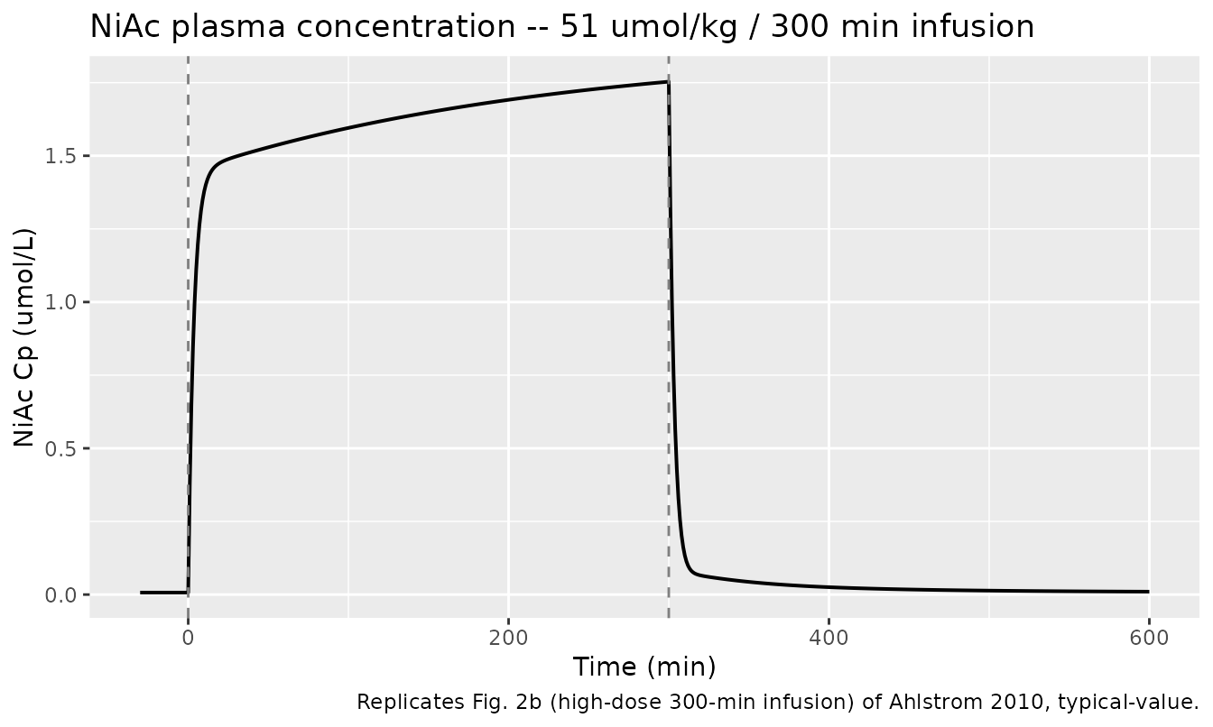
ggplot(sim_300, aes(time, NEFA)) +
  geom_line(linewidth = 0.7) +
  geom_hline(yintercept = 0.606, linetype = "dotted", colour = "grey50") +
  geom_vline(xintercept = c(0, 300), linetype = "dashed", colour = "grey50") +
  labs(x = "Time (min)", y = "NEFA (mmol/L)",
       title = "NEFA response -- 51 umol/kg / 300 min infusion",
       caption = paste("Replicates Fig. 6b / Fig. 7b (NEFA after 300-min infusion) of",
                       "Ahlstrom 2010. Tolerance develops during the infusion (NEFA",
                       "recovers from its early nadir even though NiAc is still being",
                       "infused); after cessation, NEFA rebounds above baseline."))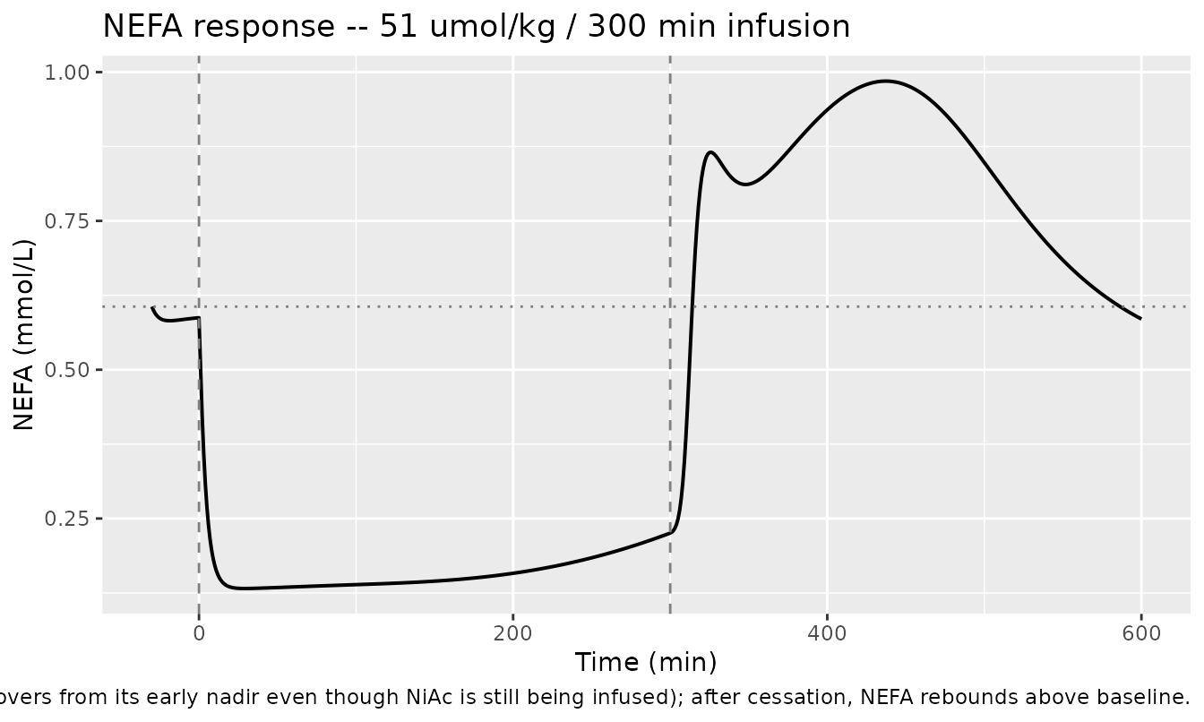
Steady-state equilibrium relationship (Fig. 9)
Figure 9 of Ahlstrom 2010 plots the steady-state NEFA response vs. plasma NiAc concentration for the tolerant system (Eq. 15) and for the non-tolerant system (Eq. 17). We reproduce the curves by sweeping a constant continuous infusion that yields a target Cp at steady-state, then reading NEFA at the very end of the simulation (after the moderator chain has fully equilibrated).
typical <- list(
  r0     = 0.606,
  kout   = 0.411,
  ic50   = 0.0446,
  gam    = 1.48,
  pmod   = 1.21,
  kcap   = 0.0318,
  imax   = 1
)

# Closed-form tolerant Rss (paper Eq. 15): solves
#   0 = kin*(1 - I(Cp)) / Rss^p + kcap - kout * Rss^2
# numerically for a grid of Cp.
inh <- function(Cp, par) par$imax * Cp^par$gam / (par$ic50^par$gam + Cp^par$gam)
solve_rss_tol <- function(Cp, par) {
  kin <- par$r0^par$pmod * (par$kout * par$r0^2 - par$kcap)
  f <- function(R) kin * (1 - inh(Cp, par)) / R^par$pmod + par$kcap -
                    par$kout * R^2
  uniroot(f, lower = 1e-4, upper = 5)$root
}
# Closed-form non-tolerant Rss (paper Eq. 17): no moderator amplification.
solve_rss_notol <- function(Cp, par) {
  kin <- par$kout * par$r0^2 - par$kcap
  f <- function(R) kin * (1 - inh(Cp, par)) + par$kcap - par$kout * par$r0 * R
  uniroot(f, lower = 1e-4, upper = 5)$root
}

Cp_grid <- 10^seq(-3.5, 2, length.out = 80)
fig9 <- tibble(
  Cp        = Cp_grid,
  Rss_tol   = sapply(Cp_grid, solve_rss_tol,   par = typical),
  Rss_notol = sapply(Cp_grid, solve_rss_notol, par = typical)
) |>
  tidyr::pivot_longer(c(Rss_tol, Rss_notol), names_to = "system", values_to = "Rss")

ggplot(fig9, aes(Cp, Rss, linetype = system)) +
  geom_line(linewidth = 0.7) +
  scale_x_log10() +
  scale_linetype_manual(values = c(Rss_tol = "solid", Rss_notol = "dashed"),
                        labels = c(Rss_tol = "Tolerant (Eq. 15)",
                                   Rss_notol = "Non-tolerant (Eq. 17)")) +
  labs(x = "NiAc Cp (umol/L, log scale)", y = "NEFA Rss (mmol/L)",
       linetype = NULL,
       title = "Steady-state NiAc concentration vs NEFA response",
       caption = "Replicates Fig. 9 of Ahlstrom 2010. Tolerant curve is shifted to the right and is shallower than the non-tolerant curve.")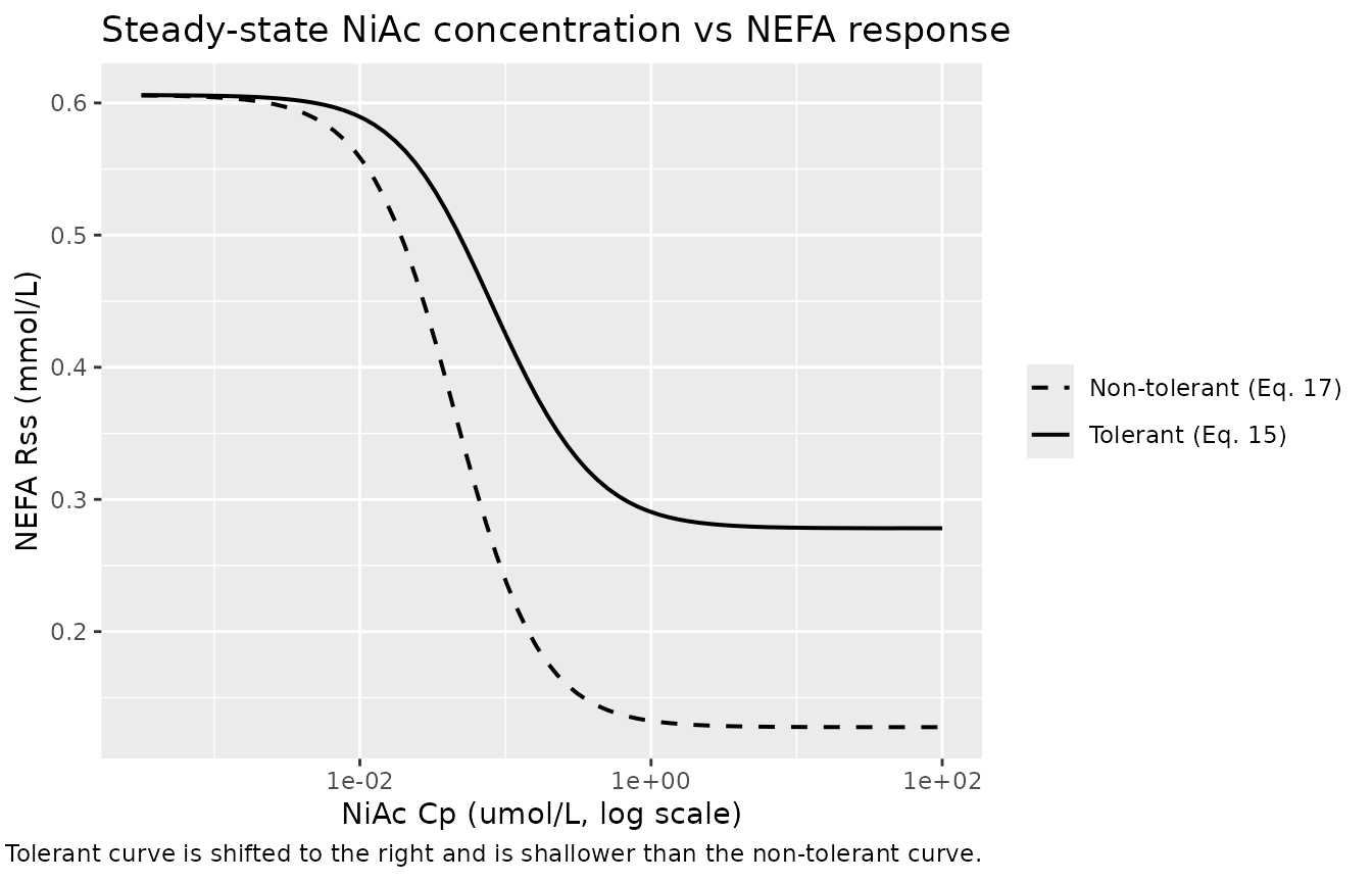
Endogenous baseline check (Cp at no-drug steady state)
With Inf = 0 the central-compartment balance reduces to a quadratic
in Cp_baseline (Appendix A Eqs. 9-12). The model file solves the
quadratic inline and uses its positive root as the initial condition for
the central and peripheral1 states, so the
typical-value Cp at t = 0 should equal the paper’s reported endogenous
estimate (6.8 nmol/L).
The paper’s kin = R0^p * (kout * R0^2 - kcap) formula is
derived assuming I(Cp) = 0 (no drug), so the model has a small baseline
drift in NEFA when endogenous NiAc is nonzero: at endogenous Cp ~ 6.8
nmol/L and IC50 = 44.6 nmol/L, I(Cp) ~ 6%, which suppresses NEFA
formation slightly below R0. The system’s natural attractor at
endogenous Cp is ~0.59 mmol/L rather than exactly R0 = 0.606. This is a
self-consistent property of the published model, not a translation error
– see “Assumptions and deviations” below.
ev_baseline <- make_events(dose_umolkg = 0, dur_min = 0, tmax = 120, dt = 5)
sim_b <- as.data.frame(rxSolve(mod_typical, ev_baseline))
#> ℹ omega/sigma items treated as zero: 'etalvmax_lo', 'etalq', 'etalsynt', 'etalrbase', 'etalkout', 'etalic50'
Cp_baseline_nm <- sim_b$Cc[sim_b$time == 0][1] * 1000   # nmol/L
NEFA_t0        <- sim_b$NEFA[sim_b$time == 0][1]
cat(sprintf("Cp_baseline (typical) = %s nmol/L (paper: 6.80 nmol/L)\n",
            format(signif(Cp_baseline_nm, 3))))
#> Cp_baseline (typical) = 6.83 nmol/L (paper: 6.80 nmol/L)
cat(sprintf("NEFA at t = 0 (typical) = %s mmol/L (R0 = 0.606; ~%.1f%% below R0)\n",
            format(signif(NEFA_t0, 4)),
            100 * (0.606 - NEFA_t0) / 0.606))
#> NEFA at t = 0 (typical) = 0.5873 mmol/L (R0 = 0.606; ~3.1% below R0)
stopifnot(abs(Cp_baseline_nm - 6.8) < 0.1)
stopifnot(NEFA_t0 > 0.55 && NEFA_t0 < 0.61)
Mass-balance / steady-state hold
With no NiAc input, the NiAc compartments (Cp / Ct) hold at their endogenous baseline indefinitely (the central-compartment quadratic sets the initial condition exactly). The NEFA + moderator chain performs a small transient (~6% of R0) as it equilibrates from the R0 initial condition to the natural attractor under endogenous NiAc inhibition, after which it holds steady. We check that the NiAc holds flat and that NEFA converges to a stable value within the integration window.
ev_hold <- make_events(dose_umolkg = 0, dur_min = 0, tmax = 1440, dt = 30)
sim_hold <- as.data.frame(rxSolve(mod_typical, ev_hold))
#> ℹ omega/sigma items treated as zero: 'etalvmax_lo', 'etalq', 'etalsynt', 'etalrbase', 'etalkout', 'etalic50'
range_Cc <- range(sim_hold$Cc, na.rm = TRUE)
# NEFA equilibrates after the moderator chain (~8 / ktol ~ 300 min);
# evaluate the tail of the simulation for steady-state stability.
nefa_tail <- sim_hold$NEFA[sim_hold$time >= 720]
nefa_drift <- diff(range(nefa_tail, na.rm = TRUE))
cat(sprintf("Cc range over 24 h: [%g, %g] umol/L\n", range_Cc[1], range_Cc[2]))
#> Cc range over 24 h: [0.006829, 0.006829] umol/L
cat(sprintf("NEFA range over 12-24 h tail: %g mmol/L (max - min)\n", nefa_drift))
#> NEFA range over 12-24 h tail: 0.0004404 mmol/L (max - min)
stopifnot(diff(range_Cc) < 1e-5)
stopifnot(nefa_drift < 1e-3)
Perturbation recovery
If NEFA is displaced from baseline, the model should return to R0
over many half-lives of the slower (moderator) process, with damped
oscillations expected at the chosen p exponent.
ev_pert <- make_events(dose_umolkg = 0, dur_min = 0, tmax = 1500, dt = 5)
sim_low  <- as.data.frame(rxSolve(mod_typical, ev_pert,
                                  inits = c(nefa = 0.3 * 0.606)))
#> ℹ omega/sigma items treated as zero: 'etalvmax_lo', 'etalq', 'etalsynt', 'etalrbase', 'etalkout', 'etalic50'
sim_high <- as.data.frame(rxSolve(mod_typical, ev_pert,
                                  inits = c(nefa = 2.0 * 0.606)))
#> ℹ omega/sigma items treated as zero: 'etalvmax_lo', 'etalq', 'etalsynt', 'etalrbase', 'etalkout', 'etalic50'
bind_rows(
  sim_low  |> mutate(scenario = "Start at 0.3 x R0"),
  sim_high |> mutate(scenario = "Start at 2.0 x R0")
) |>
  ggplot(aes(time, NEFA, colour = scenario)) +
  geom_line(linewidth = 0.7) +
  geom_hline(yintercept = 0.606, linetype = "dotted") +
  labs(x = "Time (min)", y = "NEFA (mmol/L)", colour = NULL,
       title = "Perturbation recovery of NEFA",
       caption = "Damped return to R0 with characteristic time set by the moderator chain (8 transit cmts, ktol = 0.0267 1/min).")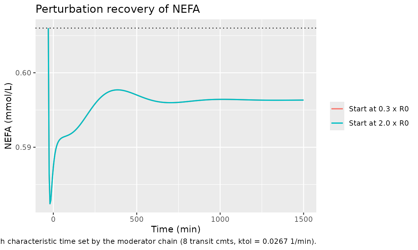
Virtual cohort – between-subject variability
set.seed(1)
n_subj <- 30
# Build matched cohort: each subject receives a dose-by-duration regimen.
regimens <- tibble::tribble(
  ~regimen,                ~dose_umolkg, ~dur_min,
  "5 umol/kg / 30 min",    5,            30,
  "20 umol/kg / 30 min",   20,           30,
  "10 umol/kg / 300 min",  10,           300,
  "51 umol/kg / 300 min",  51,           300
)
build_regimen_events <- function(regimens, n_per, tmax = 600, dt = 5) {
  out <- vector("list", nrow(regimens))
  off <- 0L
  for (i in seq_len(nrow(regimens))) {
    rg <- regimens[i, ]
    for (k in seq_len(n_per)) {
      ev_k <- make_events(dose_umolkg = rg$dose_umolkg,
                          dur_min     = rg$dur_min,
                          tmax        = tmax,
                          dt          = dt,
                          id_offset   = off + k - 1L)
      ev_k$regimen <- rg$regimen
      out[[length(out) + 1]] <- ev_k
    }
    off <- off + n_per
  }
  dplyr::bind_rows(out)
}
events_cohort <- build_regimen_events(regimens, n_per = n_subj %/% nrow(regimens),
                                      tmax = 600, dt = 5)
stopifnot(!anyDuplicated(unique(events_cohort[, c("id", "time", "evid", "cmt")])))

sim_cohort <- rxode2::rxSolve(mod, events_cohort,
                              keep = c("regimen")) |>
  as.data.frame()
#> ℹ parameter labels from comments will be replaced by 'label()'

sim_cohort |>
  dplyr::filter(time >= -30) |>
  group_by(regimen, time) |>
  summarise(med = median(NEFA, na.rm = TRUE),
            lo  = quantile(NEFA, 0.10, na.rm = TRUE),
            hi  = quantile(NEFA, 0.90, na.rm = TRUE),
            .groups = "drop") |>
  ggplot(aes(time, med)) +
  geom_ribbon(aes(ymin = lo, ymax = hi), alpha = 0.25) +
  geom_line(linewidth = 0.7) +
  facet_wrap(~regimen) +
  geom_hline(yintercept = 0.606, linetype = "dotted") +
  labs(x = "Time (min)", y = "NEFA (mmol/L)",
       title = "Virtual cohort -- NEFA trajectories with IIV",
       caption = "Median (line) and 10-90% spread (ribbon) over the virtual cohort.")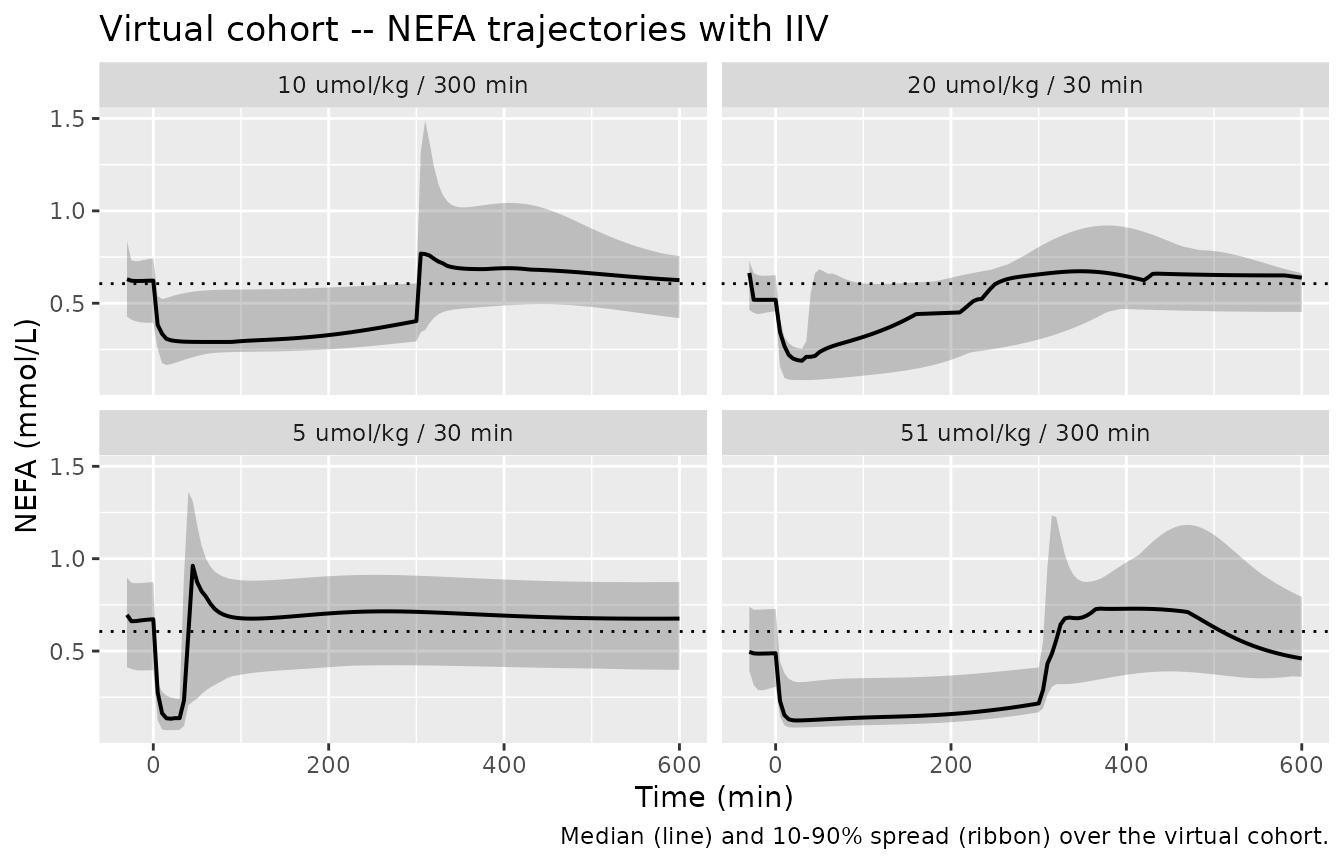
Assumptions and deviations
-
Body-weight scaling. The paper reports all PK
parameters on a per-kg basis (Vmax, Synt in umol/min/kg; Vc, Cld, Vt in
L/kg) and the PD model has no covariates. The model file follows the
same per-kg parameterisation:
amt = 20in the event table means 20 umol/kg of body weight, and Cp is computed from amount / Vc per kg. A user with an actual rat body weight can either work in per-kg units directly or multiply Vmax/Synt/Q/Vc/Vp by body weight to switch to absolute units – the model is invariant to that re-scaling because every flux term inherits the per-kg dimension consistently. - Endogenous baseline. The central and peripheral compartment initial conditions are set from the analytic positive root of the baseline quadratic (paper Appendix A Eq. 12). For the typical-value parameter set this yields Cp_baseline = 6.8 nmol/L, matching the paper’s reported endogenous estimate; individual rats with different draws of (Synt, Vmax2) get individual baselines spanning roughly 4.8-15 nmol/L (Results), reproducing the paper’s population range. For an individual draw where the quadratic discriminant becomes marginal (very low Vmax2 or high Synt simultaneously) the solver may produce a non-physical value – such draws are rare under the reported IIVs and the user should screen the simulated cohort if a small fraction of unphysical baselines becomes a problem.
-
NEFA
kin. The turnover-rate inputkinis computed per the published formulaR0^p * (kout * R0^2 - kcap)(text following Eq. 4). This formula is derived by setting I(Cp) = 0 in Eq. 3 at baseline, so it implicitly assumes that the endogenous NiAc plasma concentration is negligible relative to IC50. In reality endogenous Cp ~ 6.8 nmol/L is non-zero, IC50 = 44.6 nmol/L, and the implied baseline inhibition is I(Cp_endogenous) ~ 6%. The model file reproduces the paper’s formula verbatim; the consequence is that the NEFA + moderator system’s true steady state under endogenous NiAc is approximately 6% below R0 (~0.59 mmol/L typical), not exactly R0 = 0.606. This is a self-consistent property of the published model (R0 in the paper is the formula’s no-drug baseline parameter, fit to data that the authors treated as predose / endogenous-Cp baseline) – it is not a translation error and should not be “corrected” by inflating kin to absorb endogenous inhibition. The baseline drift is small relative to the experimental NEFA variability (range 0.3-1.1 mmol/L per Results) and disappears quickly relative to the drug-induced response.- For unusual individual draws with very low kout and high kcap, the
bracket
(kout * R0^2 - kcap)can be small or negative – which would produce a non-physical kin. Under the reported IIVs this is an extreme-tail event; the vignette’s typical-value plots and the median/10-90% cohort ribbons are not affected.
- For unusual individual draws with very low kout and high kcap, the
bracket
-
Compartment naming. The 8 moderator transit
compartments use the blessed
precursor<n>chain prefix because that is the closest existing nlmixr2lib convention for a first-order delay cascade (see also Friberg 2002 paclitaxel, which uses the same prefix for a feedback chain of biological precursors). The model file is explicit that these correspond to the paper’s M1..M8 moderator compartments. A new lowercase compartmentnefais registered alongside this model inR/conventions.R(sibling toglucose/lactatealready in that list). -
Residual-error unit for the NiAc additive term.
Ahlstrom 2010 Table 1 reports the additive PK residual error as
r2 (%) = 0.800. Additive residual error cannot meaningfully be a percent; the(%)header is a typographic artefact (it is the units header inherited from the row above,r1 (%) = 34.4proportional CV%). The model encodes the value literally asaddSd = 0.800on the assumption that the implicit unit is umol/L (the NONMEM data unit used throughout the paper, given NiAc plasma concentrations are reported in umol/L and range 0.001-20 umol/L). This residual layer is informational and does not affect the typical-value simulations in this vignette. -
No PKNCA validation block. The Ahlstrom model is a
coupled PKPD feedback system with an endogenous PK baseline (NiAc has
nonzero steady-state plasma from continuous Synt synthesis) and a
non-monotonic NEFA response (suppression, tolerance, rebound,
oscillations). NCA on either output is not a meaningful validation
target – the paper itself does not report NCA parameters. Validation
here is done via (1) steady-state hold, (2) perturbation recovery,
- Fig. 2 / Fig. 6 figure replication, and (4) the Fig. 9 steady-state response curve.
- Errata. No erratum or corrigendum was identified for this paper as of the model extraction date.