Teicoplanin (Butragueno-Laiseca 2025)
Source:vignettes/articles/ButraguenoLaiseca_2025_teicoplanin.Rmd
ButraguenoLaiseca_2025_teicoplanin.RmdModel and source
ui <- rxode2::rxode(readModelDb("ButraguenoLaiseca_2025_teicoplanin"))
#> ℹ parameter labels from comments will be replaced by 'label()'- Citation: Butragueno-Laiseca L, Garcia-Orueta G, Riva N, Troconiz IF, Fernandez SN, Camacho Vicente V, Padilla B, Slocker M, Santiago MJ. Population pharmacokinetic analysis of teicoplanin in paediatric patients, including those receiving continuous kidney replacement therapy: a prospective cohort study. J Antimicrob Chemother. 2025;80(3):868-875. doi:10.1093/jac/dkaf012.
- Description: Two-compartment population PK model for intravenous teicoplanin in 26 critically ill children in a paediatric ICU, 12 of whom were receiving continuous kidney replacement therapy (CKRT) in continuous venovenous haemodiafiltration modality (Butragueno-Laiseca 2025). Plasma, pre-filter and post-filter concentrations were fitted simultaneously. Elimination from the central compartment is partitioned into a renal arm (CLR, 0.169 L/h typical at 8 kg, allometrically scaled with a fixed exponent of 0.75, encoded as lcl_renal) and a haemofilter arm (CLKRT, 0.119 L/h typical for the small filter, encoded as lcl_hemodialysis). The two arms are mutually exclusive: renal clearance was estimated to be zero while CKRT was running, so total clearance is CLR off CKRT and CLKRT on CKRT. Haemofilter surface area is a categorical covariate on the CKRT arm (small 0.2 m2 reference; medium 0.6 m2 multiplier 3.58; large 1.2 m2 multiplier 5.04). Central volume scales allometrically with body weight with a fixed exponent of 1; the peripheral volume and the inter-compartmental clearance carry no covariates and no IIV. The post-filter concentration is derived algebraically from the pre-filter (central) concentration and the filter extraction ratio CLKRT divided by the plasma flow entering the haemofilter, and carries its own residual error. No other patient characteristic, including estimated glomerular filtration rate and serum albumin, was retained.
- Article: https://doi.org/10.1093/jac/dkaf012
- Supplement:
dkaf012_supplementary_data.docx, available from the Europe PMC open-access record for PMC11879232
Population
Twenty-six critically ill children treated with teicoplanin in a single paediatric intensive care unit (Hospital General Universitario Gregorio Maranon, Madrid) were enrolled; twelve of them were undergoing continuous kidney replacement therapy (CKRT) in continuous venovenous haemodiafiltration modality. Median (range) weight was 8 kg (4.3-44 kg) and median age 14 months (3 months to 13 years). Most patients were in the post-operative period of a congenital cardiopathy, nearly all were mechanically ventilated, and the median PRISM III score was 6 (no CKRT) and 8 (CKRT). Baseline characteristics are reported separately for the 15 patients without and the 12 with a haemofilter in Butragueno-Laiseca 2025 Table 1; the two group sizes sum to 27 rather than 26 because one patient started treatment without CKRT and required CKRT after the fifth dose, contributing to both groups (Table 1 footnote a).
All patients received the standard paediatric regimen: three loading doses of 10 mg/kg every 12 h, followed 24 h later by a maintenance dose of 10 mg/kg every 24 h (3.3 mg/kg every 24 h in CKRT patients), each given as a 5-min intravenous infusion. A total of 173 concentrations were modelled - 72 plasma samples from non-CKRT patients and 51 pre-filter plus 50 post-filter samples from CKRT patients - all above the 1.0 mg/L limit of quantification and ranging from 2.1 to 86.6 mg/L.
The same information is available programmatically via the model’s
population metadata:
str(ui$population, max.level = 1)
#> List of 14
#>  $ species       : chr "human"
#>  $ n_subjects    : int 26
#>  $ n_studies     : int 1
#>  $ n_observations: int 173
#>  $ age_range     : chr "3 months to 13 years"
#>  $ age_median    : chr "14 months"
#>  $ weight_range  : chr "4.3-44 kg"
#>  $ weight_median : chr "8 kg"
#>  $ race_ethnicity: chr "Not reported."
#>  $ disease_state : chr "Critically ill children admitted to a paediatric intensive care unit and treated with teicoplanin, 12 of them u"| __truncated__
#>  $ dose_range    : chr "Standard paediatric regimen: three loading doses of 10 mg/kg every 12 h in all patients, followed 24 h later by"| __truncated__
#>  $ regions       : chr "Hospital General Universitario Gregorio Maranon, Madrid, Spain (single centre)."
#>  $ renal_function: chr "Non-CKRT group: eGFR (bedside Schwartz) median 112 mL/min, range 29-283 mL/min; serum creatinine median 0.32 mg"| __truncated__
#>  $ notes         : chr "Baseline demographics from Butragueno-Laiseca 2025 Table 1, reported separately for the 15 patients without and"| __truncated__
Source trace
The per-parameter origin is recorded as an in-file comment next to
each ini() entry in
inst/modeldb/specificDrugs/ButraguenoLaiseca_2025_teicoplanin.R.
The table below collects them in one place for review.
| Equation / parameter | Value | Source location |
|---|---|---|
lcl_renal (theta_CLR) |
0.169 L/h | Table 2 (RSE 12%; SIR 95% CI 0.139-0.208) |
lcl_hemodialysis (theta_CLKRT) |
0.119 L/h | Table 2 (RSE 8%; SIR 95% CI 0.103-0.136) |
lvc (theta_V1) |
1.56 L | Table 2 (RSE 17%; SIR 95% CI 1.03-1.98) |
lvp (theta_V2) |
3.03 L | Table 2 (RSE 30%; SIR 95% CI 2.10-4.53) |
lq (theta_CLD) |
0.292 L/h | Table 2 (RSE 53%; SIR 95% CI 0.167-0.614) |
e_wt_cl_renal |
0.75 (fixed) | Results, Covariate selection (“exponents of 1 and 0.75 for V1 and CLR”) |
e_wt_vc |
1 (fixed) | Results, Covariate selection |
| reference weight | 8 kg | Table 2 Parameter model column (WGT/8); cohort median
weight, Results |
e_filt_sa_med_cl_hemodialysis |
3.58 | Table 2, theta_FILT Med (RSE 13%; SIR 95% CI 2.78-4.40) |
e_filt_sa_large_cl_hemodialysis |
5.04 | Table 2, theta_FILT Large (RSE 14%; SIR 95% CI 3.80-6.26) |
| theta_FILT Small = 1 (reference) | 1 | Table 2 |
etalcl_renal |
30.4% CV | Table 2 IIV column (RSE 32%; eta-shrinkage 33%) |
etalcl_hemodialysis |
14.1% CV | Table 2 IIV column (RSE 19%; eta-shrinkage 45%) |
etalvc |
39.2% CV | Table 2 IIV column (RSE 45%; eta-shrinkage 40%) |
| omega^2 = log(1 + CV^2) | n/a | Table 2 footnote (CV% = sqrt(exp(omega^2) - 1) x 100) |
expSd |
0.301 | Table 2, plasma residual error (RSE 8%; SIR 95% CI 0.27-0.34) |
expSd_Cpostfilter |
0.333 | Table 2, post-filter residual error (RSE 13%; SIR 95% CI 0.28-0.39) |
Log-additive residual -> lnorm()
|
n/a | Methods, PK analysis (“additive error model in the logarithmic scale”) |
| Two-compartment structure | n/a | Results, Base population model; Figure S2; Supplementary material (“one-compartment model performed significantly worse … three-compartment model did not improve the fit”) |
| CLNR removed | n/a | Results, Base population model (“CLNR could not be identified and was therefore removed”) |
| CLR = 0 during CKRT | n/a | Table 2 footnote a; Supplementary material, Base population model (“thus, CL equals CLKRT”) |
| No IIV on V2 / CLD; no eta covariance | n/a | Results, Base population model |
Cpostfilter = Cc * (1 - CLKRT / phi_PlCorr) |
n/a | Supplementary material, Pharmacokinetic analysis (displayed equation) |
phi_PlCorr = phi_Blood x BPR |
n/a | Supplementary material, Pharmacokinetic analysis (BPR reading documented in Errata) |
| 5-min IV infusion | n/a | Methods, Dosing sampling and analytical method |
Structural checks
These checks are deterministic consequences of the encoded parameters
and can be evaluated without simulating: each is a statement the paper
makes about its own model, recomputed from the packaged
ini() values.
th <- setNames(ui$theta, names(ui$theta))

theta_clr   <- exp(th[["lcl_renal"]])
theta_clkrt <- exp(th[["lcl_hemodialysis"]])
theta_v1    <- exp(th[["lvc"]])
ref_wt      <- 8

# Discussion: "The model predicts an increase in 0.016 L/h and 0.19 L,
# respectively, for an increment of 1 kg of body weight."
d_clr_dwt <- theta_clr * th[["e_wt_cl_renal"]] / ref_wt   # d/dWT at WT = 8 kg
d_v1_dwt  <- theta_v1  * th[["e_wt_vc"]]       / ref_wt

# Discussion: "the estimate of CLKRT (0.119 L/h) was 30% lower than CLR".
pct_lower <- 100 * (theta_clr - theta_clkrt) / theta_clr

structural <- tibble::tibble(
  Check = c(
    "dCLR/dWT at 8 kg (L/h per kg)",
    "dV1/dWT at 8 kg (L per kg)",
    "CLKRT below CLR (%)",
    "CLKRT, medium 0.6 m2 filter (L/h)",
    "CLKRT, large 1.2 m2 filter (L/h)"
  ),
  Model = c(
    d_clr_dwt, d_v1_dwt, pct_lower,
    theta_clkrt * th[["e_filt_sa_med_cl_hemodialysis"]],
    theta_clkrt * th[["e_filt_sa_large_cl_hemodialysis"]]
  ),
  Published = c(0.016, 0.19, 30, 0.119 * 3.58, 0.119 * 5.04),
  Source = c(
    "Discussion", "Discussion", "Discussion",
    "Table 2 (theta_CLKRT x theta_FILT Med)",
    "Table 2 (theta_CLKRT x theta_FILT Large)"
  )
)

# Each published figure is quoted to two significant figures, so the model
# value must fall inside the rounding interval of the printed value: within
# half a unit of the last published digit. The V1 slope is the tight case --
# 1.56 / 8 is exactly 0.195, which the paper prints as 0.19, so the model
# value sits precisely on the interval boundary and the comparison needs an
# epsilon to survive binary floating point (0.195 - 0.19 evaluates to
# 0.005000000000000004).
matches_published <- function(model, published, half_ulp) {
  abs(model - published) <= half_ulp + 1e-9
}

stopifnot(
  matches_published(d_clr_dwt, 0.016, 0.0005),
  matches_published(d_v1_dwt,  0.19,  0.005),
  matches_published(pct_lower, 30,    1)
)
# The slopes are also exact analytic consequences of the encoded parameters.
stopifnot(
  isTRUE(all.equal(d_clr_dwt, 0.169 * 0.75 / 8)),
  isTRUE(all.equal(d_v1_dwt,  1.56 / 8))
)

structural |>
  dplyr::mutate(Model = signif(Model, 3), Published = signif(Published, 3)) |>
knitr::kable(caption = "Structural consequences of the encoded parameters versus the values Butragueno-Laiseca 2025 states for its own model.")| Check | Model | Published | Source |
|---|---|---|---|
| dCLR/dWT at 8 kg (L/h per kg) | 0.0158 | 0.016 | Discussion |
| dV1/dWT at 8 kg (L per kg) | 0.1950 | 0.190 | Discussion |
| CLKRT below CLR (%) | 29.6000 | 30.000 | Discussion |
| CLKRT, medium 0.6 m2 filter (L/h) | 0.4260 | 0.426 | Table 2 (theta_CLKRT x theta_FILT Med) |
| CLKRT, large 1.2 m2 filter (L/h) | 0.6000 | 0.600 | Table 2 (theta_CLKRT x theta_FILT Large) |
The post-filter observation equation is checked the same way. With
the CKRT cohort medians of Table 1 (blood flow 50 mL/min, haematocrit
29.3%) the plasma flow entering the haemofilter is
50 x 0.06 x (1 - 0.293) = 2.12 L/h, so the single-pass
extraction ratio CLKRT / phi_PlCorr rises with filter
size:
plasma_flow <- 50 * 0.06 * (1 - 29.3 / 100)   # mL/min -> L/h, times plasma fraction

tibble::tibble(
  `Filter` = c("Small (0.2 m2)", "Medium (0.6 m2)", "Large (1.2 m2)"),
  `CLKRT (L/h)` = theta_clkrt *
    c(1, th[["e_filt_sa_med_cl_hemodialysis"]], th[["e_filt_sa_large_cl_hemodialysis"]]),
  `Extraction ratio` = theta_clkrt *
    c(1, th[["e_filt_sa_med_cl_hemodialysis"]], th[["e_filt_sa_large_cl_hemodialysis"]]) / plasma_flow
) |>
  dplyr::mutate(dplyr::across(where(is.numeric), \(x) signif(x, 3))) |>
  dplyr::mutate(`Cpost / Cpre` = signif(1 - `Extraction ratio`, 3)) |>
knitr::kable(caption = "Single-pass haemofilter extraction implied by the supplementary post-filter equation at the Table 1 median blood flow and haematocrit.")| Filter | CLKRT (L/h) | Extraction ratio | Cpost / Cpre |
|---|---|---|---|
| Small (0.2 m2) | 0.119 | 0.0561 | 0.944 |
| Medium (0.6 m2) | 0.426 | 0.2010 | 0.799 |
| Large (1.2 m2) | 0.600 | 0.2830 | 0.717 |
The resulting 6-28% single-pass extraction is consistent with the paper’s observation that post-filter concentrations are only modestly below pre-filter concentrations, and with the Discussion note that teicoplanin’s high protein binding means “theoretically only 10% of the drug should be eliminated”.
Virtual cohort
Original observed data are not publicly available. The cohort below reproduces the simulation design of Butragueno-Laiseca 2025 (Methods, Percentage of target attainment): body weight is the only covariate simulated, sampled within the three published weight bands (3-10, 11-30, 31-60 kg). Four regimens are simulated - the standard regimen and the paper’s recommended alternative, for CKRT and non-CKRT patients (Table S1).
Haemofilter size is held at the reference (small, 0.2 m2) level in these target-attainment simulations, which is how the paper ran them: “In simulations, the only covariate that was simulated was body weight, given that filter size was considered as a surrogate of body weight. Haemofilter settings were not needed to simulate plasma concentrations” (Results, Probability of target attainment). That sentence admits two readings - derive filter size from the simulated weight, or drop the filter term entirely - and they give very different answers. The published target-attainment percentages discriminate between them, and both readings are simulated side by side in Which reading of the filter-size sentence? below: holding the filter at its reference level reproduces the published values and deriving it from weight does not, so that is the design used here. The filter-size covariate is still encoded in the model - it is what Table 2 estimates - and is exercised separately in its own cohort.
set.seed(20250107)

n_per_arm <- 100L

weight_bands <- tibble::tribble(
  ~wt_group,  ~wt_lo, ~wt_hi,
  "3-10 kg",     3,     10,
  "11-30 kg",   11,     30,
  "31-60 kg",   31,     60
)

regimens <- tibble::tribble(
  ~regimen,                              ~ckrt, ~ld_mgkg, ~md_mgkg,
  "No CKRT: 3 x 10 q12h + 10 q24h",          0,       10,     10.0,
  "No CKRT: 3 x 15 q12h + 15 q24h",          0,       15,     15.0,
  "CKRT: 3 x 10 q12h + 3.3 q24h",            1,       10,      3.3,
  "CKRT: 3 x 15 q12h + 10 q24h",             1,       15,     10.0
)

arms <- tidyr::crossing(regimens, weight_bands)

# Observation grid: fine over the first hour so the 5-min infusion peak is
# resolved, then every 30 min out to the 72 h trough.
obs_times <- sort(unique(c(seq(0, 1, by = 0.05), seq(1, 72, by = 0.5))))
dose_times <- c(0, 12, 24, 48)   # 3 loading doses q12h, first maintenance 24 h later
inf_dur    <- 5 / 60             # 5-min infusion (Methods, Dosing)

make_arm <- function(regimen, ckrt, ld_mgkg, md_mgkg,
                     wt_group, wt_lo, wt_hi,
                     n = n_per_arm, id_offset = 0L) {
  subj <- tibble::tibble(
    id              = id_offset + seq_len(n),
    WT              = exp(runif(n, log(wt_lo), log(wt_hi))),
    RRT_CRRT_ACTIVE = ckrt,
    # Reference (small, 0.2 m2) haemofilter throughout -- see the note above.
    FILT_SA_MED     = 0,
    FILT_SA_LARGE   = 0,
    # Blood flow and haematocrit enter only the post-filter observation.
    # Table 1 medians (range) for the CKRT group: 50 (34-150) mL/min and
    # 29.3% (26.3-37.5%). Non-CKRT subjects carry BFR = 0 (no circuit).
    BFR             = if (ckrt == 1) exp(runif(n, log(34), log(150))) else 0,
    HCT             = runif(n, 26.3, 37.5),
    regimen         = regimen,
    wt_group        = wt_group
  )

  doses <- subj |>
    tidyr::crossing(time = dose_times) |>
    dplyr::mutate(
      amt  = WT * ifelse(time < 48, ld_mgkg, md_mgkg),
      rate = amt / inf_dur,
      evid = 1L,
      cmt  = "central",
      dvid = NA_integer_
    )

  # Both model outputs (Cc and Cpostfilter) are algebraic transforms of the
  # single `central` state, so rxode2 assigns them endpoint slots AFTER the
  # ODE states and an observation row carrying cmt = "central" cannot be
  # matched to either endpoint. Observation rows therefore select the endpoint
  # with dvid = 1 (Cc) and leave cmt unset; rxode2 returns BOTH observables as
  # columns on every observation row.
  obs <- subj |>
    tidyr::crossing(time = obs_times) |>
    dplyr::mutate(
      amt  = NA_real_, rate = NA_real_, evid = 0L,
      cmt  = NA_character_, dvid = 1L
    )

  dplyr::bind_rows(doses, obs) |>
    dplyr::arrange(id, time, dplyr::desc(evid))
}

events <- do.call(
  dplyr::bind_rows,
  lapply(seq_len(nrow(arms)), function(i) {
    a <- arms[i, ]
    do.call(make_arm, c(as.list(a), list(id_offset = (i - 1L) * n_per_arm)))
  })
)

stopifnot(!anyDuplicated(events[, c("id", "time", "evid")]))
stopifnot(length(unique(events$id)) == nrow(arms) * n_per_arm)

nrow(events)
#> [1] 200400
Simulation
mod <- readModelDb("ButraguenoLaiseca_2025_teicoplanin")

sim <- rxode2::rxSolve(
  mod,
  events = events,
  keep   = c("regimen", "wt_group", "WT", "RRT_CRRT_ACTIVE"),
  # rxode2's automatic ODE -> linCmt conversion mis-maps the endpoints of
  # multi-output models.
  useLinCmt = FALSE
) |>
  as.data.frame() |>
  dplyr::filter(!is.na(Cc))
#> ℹ parameter labels from comments will be replaced by 'label()'
Replicate published figures
sim |>
  dplyr::group_by(regimen, wt_group, time) |>
  dplyr::summarise(
    Q025 = quantile(Cc, 0.025),
    Q50  = quantile(Cc, 0.50),
    Q975 = quantile(Cc, 0.975),
    .groups = "drop"
  ) |>
  ggplot(aes(time, Q50)) +
  geom_ribbon(aes(ymin = Q025, ymax = Q975), alpha = 0.25) +
  geom_line() +
  geom_hline(yintercept = c(10, 60), linetype = "dashed", colour = "red") +
  facet_grid(wt_group ~ regimen) +
  scale_y_log10() +
  labs(
    x = "Time since first dose (h)",
    y = "Teicoplanin plasma concentration (mg/L)",
    title = "Simulated concentration-time profiles",
    caption = "Replicates the layout of Figure S1 of Butragueno-Laiseca 2025."
  ) +
  theme(strip.text = element_text(size = 7))
#> Warning in scale_y_log10(): log-10 transformation introduced infinite values.
#> log-10 transformation introduced infinite values.
#> log-10 transformation introduced infinite values.
#> log-10 transformation introduced infinite values.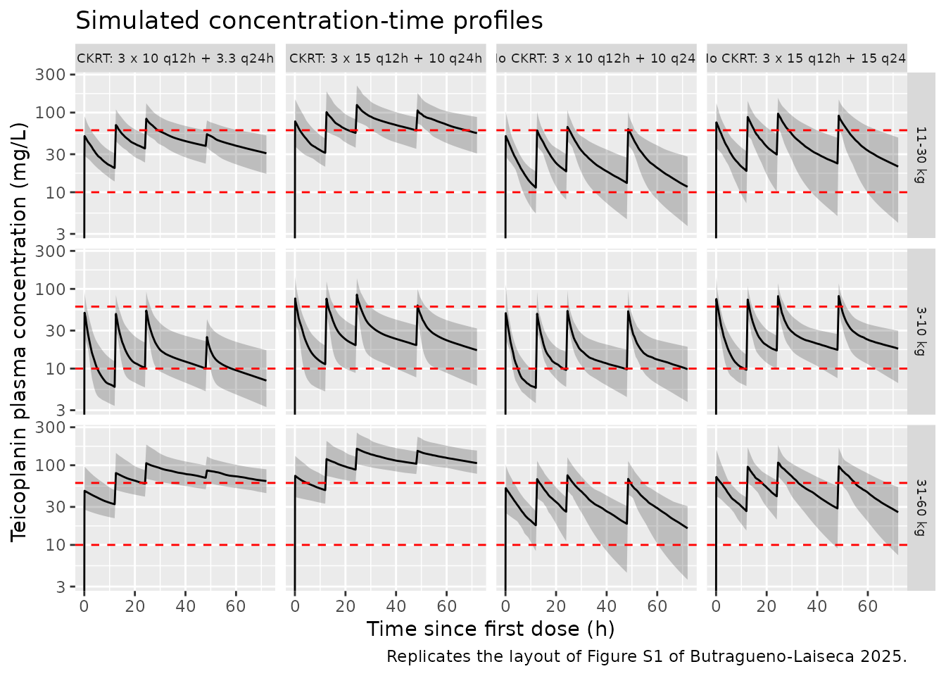
Simulated plasma concentration-time profiles by weight band and regimen. Replicates the layout of Figure S1 of Butragueno-Laiseca 2025 (median with 95% prediction interval; therapeutic range 10-60 mg/L in dashed red).
Haemofilter size and the post-filter observable
The target-attainment cohort above holds the filter at its reference size, so the filter-size covariate and the post-filter observable are exercised by a separate typical-value cohort: three subjects differing only in filter size, all at the CKRT-group median weight of 9.11 kg (Table 1) on the standard CKRT regimen, with inter-individual variability zeroed so the comparison is exact.
filter_arms <- tibble::tribble(
  ~filter,           ~FILT_SA_MED, ~FILT_SA_LARGE,
  "Small (0.2 m2)",             0,              0,
  "Medium (0.6 m2)",            1,              0,
  "Large (1.2 m2)",             0,              1
)

# Typical-value replication: IIV is zeroed so the three arms differ ONLY in
# filter size and the fold-changes can be checked exactly against Table 2
# rather than compared as medians of separately-drawn random samples.
mod_typ <- rxode2::zeroRe(mod)
#> ℹ parameter labels from comments will be replaced by 'label()'

filt_subj <- filter_arms |>
  dplyr::mutate(
    id              = dplyr::row_number(),
    WT              = 9.11,
    RRT_CRRT_ACTIVE = 1,
    BFR             = 50,
    HCT             = 29.3
  )

filt_events <- dplyr::bind_rows(
  filt_subj |>
    tidyr::crossing(time = dose_times) |>
    dplyr::mutate(
      amt = WT * ifelse(time < 48, 10, 3.3), rate = amt / inf_dur,
      evid = 1L, cmt = "central", dvid = NA_integer_
    ),
  filt_subj |>
    tidyr::crossing(time = seq(0, 72, by = 1)) |>
    dplyr::mutate(
      amt = NA_real_, rate = NA_real_, evid = 0L,
      cmt = NA_character_, dvid = 1L
    )
) |>
  dplyr::arrange(id, time, dplyr::desc(evid))

stopifnot(!anyDuplicated(filt_events[, c("id", "time", "evid")]))

sim_filt <- rxode2::rxSolve(
  mod_typ, events = filt_events, keep = "filter", useLinCmt = FALSE
) |>
  as.data.frame() |>
  dplyr::filter(!is.na(Cc), time > 0)
#> ℹ omega/sigma items treated as zero: 'etalcl_renal', 'etalcl_hemodialysis', 'etalvc'
#> Warning: multi-subject simulation without without 'omega'

filt_summary <- sim_filt |>
  dplyr::group_by(filter) |>
  dplyr::summarise(
    cl_krt   = dplyr::first(cl_hemodialysis),
    retained = dplyr::first(Cpostfilter / Cc),
    cmin72   = Cc[time == 72],
    .groups  = "drop"
  ) |>
  dplyr::mutate(filter = factor(filter, levels = filter_arms$filter)) |>
  dplyr::arrange(filter)

# With IIV zeroed these are exact identities, not approximate agreements:
# the fold-changes ARE the Table 2 theta_FILT multipliers, and the retained
# fraction IS the supplementary equation evaluated at the Table 1 medians.
cl_small <- filt_summary$cl_krt[filt_summary$filter == "Small (0.2 m2)"]
stopifnot(
  isTRUE(all.equal(cl_small, 0.119)),
  isTRUE(all.equal(
    filt_summary$cl_krt / cl_small,
    c(1, 3.58, 5.04)
  )),
  isTRUE(all.equal(
    filt_summary$retained,
    1 - filt_summary$cl_krt / plasma_flow
  ))
)

filt_summary |>
  dplyr::mutate(dplyr::across(where(is.numeric), \(x) signif(x, 3))) |>
  dplyr::rename(
    "Filter"              = filter,
    "CLKRT (L/h)"         = cl_krt,
    "Cpost / Cpre"        = retained,
    "Cmin at 72 h (mg/L)" = cmin72
  ) |>
knitr::kable(caption = "Typical-value effect of haemofilter surface area at a fixed 9.11 kg body weight on the standard CKRT regimen. Clearance rises exactly 3.58-fold (medium) and 5.04-fold (large) relative to the small reference filter -- the theta_FILT multipliers of Table 2 -- single-pass retention across the filter falls, and the 72 h trough falls with it.")| Filter | CLKRT (L/h) | Cpost / Cpre | Cmin at 72 h (mg/L) |
|---|---|---|---|
| Small (0.2 m2) | 0.119 | 0.944 | 14.400 |
| Medium (0.6 m2) | 0.426 | 0.799 | 1.460 |
| Large (1.2 m2) | 0.600 | 0.717 | 0.663 |
The retention ratios reproduce the deterministic values computed
above from the supplementary equation, and the fold-changes in
CLKRT reproduce the theta_FILT multipliers of
Table 2 exactly; both are asserted in the chunk above rather than left
to visual inspection. Note that the single-pass extraction and the
whole-body clearance are separate quantities: even a large filter
removes only about 28% of the drug per pass, but it does so
continuously, which is what makes CLKRT five times the
small-filter value.
PKNCA validation
Butragueno-Laiseca 2025 evaluates exposure over the 48-72 h window, i.e. between the first and second maintenance doses (Methods, Percentage of target attainment: “AUC24 represents the area under the plasma concentration-versus- time curve obtained between 48 and 72 h post initiation of teicoplanin therapy”). The PKNCA interval below matches that window.
sim_nca <- sim |>
  dplyr::filter(!is.na(Cc)) |>
  dplyr::select(id, time, Cc, regimen, wt_group)

conc_obj <- PKNCA::PKNCAconc(sim_nca, Cc ~ time | regimen + wt_group + id)

dose_df <- events |>
  dplyr::filter(evid == 1) |>
  dplyr::select(id, time, amt, regimen, wt_group)

dose_obj <- PKNCA::PKNCAdose(dose_df, amt ~ time | regimen + wt_group + id)

intervals <- data.frame(
  start     = 48,
  end       = 72,
  cmax      = TRUE,
  tmax      = TRUE,
  cmin      = TRUE,
  auclast   = TRUE,
  half.life = TRUE
)

nca_data <- PKNCA::PKNCAdata(conc_obj, dose_obj, intervals = intervals)
nca_res  <- PKNCA::pk.nca(nca_data)

nca_wide <- as.data.frame(nca_res) |>
  dplyr::select(regimen, wt_group, id, PPTESTCD, PPORRES) |>
  tidyr::pivot_wider(names_from = PPTESTCD, values_from = PPORRES)

nca_wide |>
  dplyr::group_by(regimen, wt_group) |>
  dplyr::summarise(
    cmax      = median(cmax),
    cmin      = median(cmin),
    auclast   = median(auclast),
    half.life = median(half.life, na.rm = TRUE),
    .groups   = "drop"
  ) |>
  dplyr::mutate(dplyr::across(where(is.numeric), \(x) signif(x, 3))) |>
  dplyr::rename(
    "Regimen"                 = regimen,
    "Weight band"             = wt_group,
    "Cmax 48-72 h (mg/L)"     = cmax,
    "Cmin 48-72 h (mg/L)"     = cmin,
    "AUC48-72 (mg*h/L)"       = auclast,
    "t1/2 (h)"                = half.life
  ) |>
knitr::kable(caption = "Median PKNCA-derived exposure over the 48-72 h dosing interval, by regimen and weight band.")| Regimen | Weight band | Cmax 48-72 h (mg/L) | Cmin 48-72 h (mg/L) | AUC48-72 (mg*h/L) | t1/2 (h) |
|---|---|---|---|---|---|
| CKRT: 3 x 10 q12h + 3.3 q24h | 11-30 kg | 53.6 | 30.80 | 947 | 39.7 |
| CKRT: 3 x 10 q12h + 3.3 q24h | 3-10 kg | 24.9 | 7.07 | 251 | 28.4 |
| CKRT: 3 x 10 q12h + 3.3 q24h | 31-60 kg | 85.9 | 63.30 | 1750 | 65.0 |
| CKRT: 3 x 15 q12h + 10 q24h | 11-30 kg | 106.0 | 55.00 | 1800 | 39.7 |
| CKRT: 3 x 15 q12h + 10 q24h | 3-10 kg | 62.0 | 17.00 | 628 | 29.4 |
| CKRT: 3 x 15 q12h + 10 q24h | 31-60 kg | 152.0 | 103.00 | 3000 | 65.2 |
| No CKRT: 3 x 10 q12h + 10 q24h | 11-30 kg | 61.9 | 11.70 | 600 | 17.1 |
| No CKRT: 3 x 10 q12h + 10 q24h | 3-10 kg | 52.4 | 9.77 | 376 | 28.1 |
| No CKRT: 3 x 10 q12h + 10 q24h | 31-60 kg | 67.4 | 16.20 | 757 | 14.5 |
| No CKRT: 3 x 15 q12h + 15 q24h | 11-30 kg | 91.4 | 21.00 | 956 | 18.1 |
| No CKRT: 3 x 15 q12h + 15 q24h | 3-10 kg | 81.4 | 17.10 | 673 | 30.3 |
| No CKRT: 3 x 15 q12h + 15 q24h | 31-60 kg | 97.1 | 25.70 | 1190 | 15.5 |
The terminal half-life recovered over this interval is consistent
with the paper’s rationale for once-daily maintenance dosing (“one of
the main advantages of teicoplanin, its relatively long half-life,
allowing once-daily dosing”, Discussion). The paper does not tabulate
NCA parameters, so no ncaComparisonTable() row-by-row
comparison is possible; the published quantities that are
numeric are the target-attainment percentages compared below.
Comparison against published target attainment
The paper reports the percentage of simulated patients reaching a trough concentration above 10 mg/L at 72 h under the standard regimen, and the AUC24/MIC > 800 target at an MIC of 1 mg/L.
cmin72 <- sim |>
  dplyr::filter(abs(time - 72) < 1e-8) |>
  dplyr::select(id, regimen, wt_group, Cmin72 = Cc)

pta <- nca_wide |>
  dplyr::left_join(cmin72, by = c("id", "regimen", "wt_group")) |>
  dplyr::group_by(regimen) |>
  dplyr::summarise(
    `PTA Cmin > 10 mg/L (%)`      = 100 * mean(Cmin72 > 10),
    `PTA Cmin > 15 mg/L (%)`      = 100 * mean(Cmin72 > 15),
    `PTA AUC24/MIC > 800, MIC 1 (%)` = 100 * mean(auclast > 800),
    `Cmin > 60 mg/L (toxicity, %)`   = 100 * mean(Cmin72 > 60),
    .groups = "drop"
  )

published_pta <- tibble::tribble(
  ~regimen,                            ~`Published PTA Cmin > 10 mg/L (%)`, ~`Published source`,
  "No CKRT: 3 x 10 q12h + 10 q24h",    66,   "Discussion (mean across weight groups)",
  "No CKRT: 3 x 15 q12h + 15 q24h",    NA,   "Figure 3a: > 90% target",
  "CKRT: 3 x 10 q12h + 3.3 q24h",      84,   "Discussion (mean across weight groups)",
  "CKRT: 3 x 15 q12h + 10 q24h",       NA,   "Figure 3b: > 90% target"
)

pta |>
  dplyr::left_join(published_pta, by = "regimen") |>
  dplyr::mutate(dplyr::across(where(is.numeric), \(x) signif(x, 3))) |>
  dplyr::rename("Regimen" = regimen) |>
knitr::kable(caption = "Simulated versus published probability of target attainment. Published values for the standard regimens are the cross-weight-group means quoted in the Discussion; for the recommended regimens the paper states only that target attainment exceeds 90% (Figure 3).")| Regimen | PTA Cmin > 10 mg/L (%) | PTA Cmin > 15 mg/L (%) | PTA AUC24/MIC > 800, MIC 1 (%) | Cmin > 60 mg/L (toxicity, %) | Published PTA Cmin > 10 mg/L (%) | Published source |
|---|---|---|---|---|---|---|
| CKRT: 3 x 10 q12h + 3.3 q24h | 77.0 | 68.7 | 54.3 | 19.700 | 84 | Discussion (mean across weight groups) |
| CKRT: 3 x 15 q12h + 10 q24h | 96.0 | 85.7 | 74.7 | 46.000 | NA | Figure 3b: > 90% target |
| No CKRT: 3 x 10 q12h + 10 q24h | 61.3 | 33.3 | 20.0 | 0.000 | 66 | Discussion (mean across weight groups) |
| No CKRT: 3 x 15 q12h + 15 q24h | 90.7 | 72.3 | 59.0 | 0.333 | NA | Figure 3a: > 90% target |
Both standard regimens reproduce the paper’s headline conclusion and
its numbers: 61% versus a published 66% without a haemofilter, and 77%
versus a published 84% with one, both short of the 90% threshold the
authors adopt. The two recommended regimens clear that threshold (91%
and 96%), matching the paper’s proposal of
3 x 15 mg/kg q12h + 15 mg/kg q24h for children without CKRT
and 3 x 15 mg/kg q12h + 10 mg/kg q24h for children on
CKRT.
The counter-intuitive ordering - CKRT patients attaining the trough
target more often than non-CKRT patients despite receiving a
third of the maintenance dose - is a property of the published model,
not an artifact: CLKRT carries no allometric term, so it
stays at 0.119 L/h regardless of body size, while CLR grows
as WT^0.75. Heavier children on CKRT therefore accumulate,
and the simulation reproduces the paper’s corresponding safety warning
that “to prevent Cmin > 60 mg/L, a loading dose exceeding 15 mg/kg in
patients weighing more than 10 kg undergoing haemofiltration should be
avoided” (Discussion): 20% of simulated CKRT patients exceed 60 mg/L on
the standard regimen and 46% on the recommended one, entirely from the
two heavier weight bands, whereas no non-CKRT regimen approaches that
threshold.
The AUC24/MIC > 800 attainment shown here is a simulated quantity and is not comparable to the 0% and 3.7% the paper reports for its 26 observed patients, who carried their real filter sizes and covariates rather than the reference-filter simulation design.
Exact agreement with the published percentages is not expected: the paper simulated 1000 profiles per scenario from its own weight distribution (Figure S1), which is not published in numeric form, whereas this vignette samples weight log-uniformly within each published band and uses 100 subjects per arm. Both standard-regimen percentages land within about 8 points of the published values, and both recommended regimens reproduce the paper’s conclusion that they clear the 90% threshold for a trough above 10 mg/L.
Which reading of the filter-size sentence?
The cohort above holds the haemofilter at its reference (small) size.
The alternative reading of the paper’s sentence - that filter size was
derived from the simulated weight, since the paper assigned
filter size by weight band (small 3-10 kg, medium 10-30 kg, large 30-60
kg; Results, Patient population) - is simulated here on exactly the same
subjects, so the two readings differ only in the value of
FILT_SA_MED / FILT_SA_LARGE.
filter_by_band <- tibble::tribble(
  ~wt_group,  ~med_derived, ~large_derived,
  "3-10 kg",             0,              0,
  "11-30 kg",            1,              0,
  "31-60 kg",            0,              1
)

# Same CKRT subjects, same weights, same dosing -- only the filter indicators
# change, so this is a paired comparison rather than a re-simulation.
events_derived <- events |>
  dplyr::filter(RRT_CRRT_ACTIVE == 1) |>
  dplyr::left_join(filter_by_band, by = "wt_group") |>
  dplyr::mutate(FILT_SA_MED = med_derived, FILT_SA_LARGE = large_derived) |>
  dplyr::select(-med_derived, -large_derived)

stopifnot(
  nrow(events_derived) == sum(events$RRT_CRRT_ACTIVE == 1),
  !anyNA(events_derived$FILT_SA_MED),
  !anyNA(events_derived$FILT_SA_LARGE)
)

pta_derived <- rxode2::rxSolve(
  mod, events = events_derived,
  keep = c("regimen", "wt_group"), useLinCmt = FALSE
) |>
  as.data.frame() |>
  dplyr::filter(!is.na(Cc), abs(time - 72) < 1e-8) |>
  dplyr::group_by(regimen) |>
  dplyr::summarise(derived = 100 * mean(Cc > 10), .groups = "drop")

published_disc <- tibble::tribble(
  ~regimen,                        ~published, ~published_label,
  "CKRT: 3 x 10 q12h + 3.3 q24h",          84, "84 (Discussion)",
  "CKRT: 3 x 15 q12h + 10 q24h",           90, "> 90 (Figure 3b)"
)

discriminator <- pta |>
  dplyr::select(regimen, reference = `PTA Cmin > 10 mg/L (%)`) |>
  dplyr::inner_join(pta_derived, by = "regimen") |>
  dplyr::inner_join(published_disc, by = "regimen")

# The design decision this table justifies: for the standard CKRT regimen --
# the one scenario with a published point estimate rather than a ">= 90%"
# statement -- the reference-filter reading must be the closer of the two.
std <- discriminator |>
  dplyr::filter(regimen == "CKRT: 3 x 10 q12h + 3.3 q24h")
stopifnot(
  nrow(std) == 1L,
  abs(std$reference - std$published) < abs(std$derived - std$published)
)

discriminator |>
  dplyr::mutate(dplyr::across(c(reference, derived), \(x) signif(x, 3))) |>
  dplyr::select(-published) |>
  dplyr::rename(
    "Regimen"                              = regimen,
    "Filter held at reference (%)"         = reference,
    "Filter derived from weight band (%)"  = derived,
    "Published (%)"                        = published_label
  ) |>
knitr::kable(caption = "The two readings of the paper's filter-size sentence, simulated on the same subjects. Holding the filter at its reference size reproduces the published target attainment; deriving it from the weight band does not.")| Regimen | Filter held at reference (%) | Filter derived from weight band (%) | Published (%) |
|---|---|---|---|
| CKRT: 3 x 10 q12h + 3.3 q24h | 77 | 23.7 | 84 (Discussion) |
| CKRT: 3 x 15 q12h + 10 q24h | 96 | 67.3 | > 90 (Figure 3b) |
Deriving the filter from weight costs 30-55 percentage points of
target attainment because CLKRT carries no allometric term
of its own, so a medium or large filter multiplies clearance 3.6- or
5-fold in exactly the heavier children whose weight-proportional dose
would otherwise have compensated. The residual gap between the
reference-filter simulation and the published 84% is attributable to the
weight distribution: this vignette samples log-uniformly within each
band, while the paper sampled from its own (non-published) distribution
shown in Figure S1.
Assumptions and deviations
-
Post-filter plasma flow (
BPR). The supplementary equation isCpost = Cpre * (1 - CLKRT / phi_PlCorr)withphi_PlCorr = phi_Blood x BPR, where BPR is described only as the “blood to plasma ratio”; the paper does not print its numerical definition. It is encoded here as the plasma fraction of blood,1 - HCT/100, which is the reading that makes the Results statement that “CKRT parameters and haematocrit were included in the model” true of this equation, and which yields physically plausible single-pass extraction ratios of 6-28% across the three filter sizes. -
Numerical floors in the post-filter equation.
model()clamps the plasma flow to a minimum of 0.001 L/h and the retained fraction1 - CLKRT/phi_PlCorrto a minimum of 0.001. Neither floor binds anywhere in the covariate ranges the paper reports; they exist so that non-CKRT subjects (who have no extracorporeal circuit and thereforeBFR = 0) do not divide by zero, and so that an extreme sampled combination of a large filter with a low blood flow cannot produce a negative concentration. - Residual-error units. Table 2 labels the residual-error rows “Residual error, log (mg/mL)”. A residual standard deviation on the log scale is unitless, and every concentration in the paper is reported in mg/L; the “(mg/mL)” label is treated as a reporting slip and the values 0.301 and 0.333 are encoded as log-scale (lnorm) residual SDs.
-
Number of observations. The Abstract states 172
concentration measurements while the Results state 173. The Results
figure is the one consistent with the reported breakdown (72 plasma + 51
pre-filter + 50 post-filter = 173) and is the value recorded in the
model’s
populationmetadata. -
Allometric exponents encoded as fixed. The
exponents of 0.75 (CLR) and 1 (V1) are reported in the Results text as
values the authors “incorporated” into the allometric expression, and
Table 2 gives no RSE or confidence interval for either, so both are
wrapped in
fixed(). -
Pre-filter and plasma concentrations share one
prediction. The paper estimates one residual magnitude for the
combined “plasma/pre-filter” group and a second for post-filter samples,
so
Ccrepresents both the plasma and the pre-filter concentration andCpostfilteris the separate post-filter observable. - Haemofilter size in the target-attainment simulations. The paper states that “the only covariate that was simulated was body weight, given that filter size was considered as a surrogate of body weight”, which could mean either that filter size was derived from the simulated weight or that the filter term was not applied at all. The two readings give target-attainment percentages roughly 30 points apart, and only the second reproduces the published values (see the Virtual cohort section for the side-by-side comparison), so the target-attainment cohort holds the filter at its reference (small) level. This affects only the vignette’s simulation design: the model file encodes the filter-size covariate exactly as Table 2 reports it, and a separate cohort exercises it.
- Cohort covariate distributions. Body weight is sampled log-uniformly within the three published weight bands; the paper’s own weight distribution (Figure S1) is not published numerically. Blood flow is set to the Table 1 median in the filter-size cohort and sampled log-uniformly over the Table 1 range (34-150 mL/min) and haematocrit uniformly over the CKRT-group range (26.3-37.5%); neither affects the plasma predictions, only the post-filter observable.
-
Target-attainment simulations use
Cc(the individual prediction) rather than a residual-error-perturbed observation. The paper does not state whether its target-attainment calculation included residual variability. - Sex, race and ethnicity are not covariates. Sex percentages are reported per group only (75% male without and 40% male with a haemofilter) and no overall value is given; race and ethnicity are not reported.