Rivaroxaban integrated multi-indication popPK (Willmann 2018a)
Source:vignettes/articles/Willmann_2018a_rivaroxaban.Rmd
Willmann_2018a_rivaroxaban.Rmd
ui <- rxode2::rxode(readModelDb("Willmann_2018a_rivaroxaban"))
#> ℹ parameter labels from comments will be replaced by 'label()'
Model and source
- Citation: Willmann S, Zhang L, Frede M, Kubitza D, Mueck W, Schmidt S, Solms A, Yan X, Garmann D. Integrated Population Pharmacokinetic Analysis of Rivaroxaban Across Multiple Patient Populations. CPT Pharmacometrics Syst Pharmacol. 2018;7(5):309-320. doi:10.1002/psp4.12288
- Article: https://doi.org/10.1002/psp4.12288 (PMC5980303, open access)
Willmann 2018a is the first integrated population PK model for rivaroxaban across all of its approved adult indications, and the first such model for any direct oral anticoagulant. It pools 22,843 concentrations from 4,918 patients in six phase II studies and one phase III substudy, and replaces the earlier per-indication models with a single covariate parameterisation.
Two source documents were used, both retrieved from EuropePMC:
- the main article (Tables 1-3, Figures 1-4), and
- the supplementary material, which supplies Supplementary
Equation 1 (the full written-out model) and, as Supplementary
Data S9, the NONMEM control stream for
run12– the final model of Table 2.
The control stream is what makes this extraction unambiguous: it
fixes the covariate centering constants, the exact form of the
dose-dependent bioavailability, the multiplicative structure of the
comedication term, the mg -> ug unit conversion, and the
residual-error form. Its $THETA,
$OMEGA and $SIGMA blocks are initial
estimates, not final ones, and are not used for any value here
– see Errata.
There is no erratum or corrigendum for this article (checked against
Crossref relation / update-to metadata and a
EuropePMC correction search).
Population
pop <- ui$population
str(pop)
#> List of 13
#>  $ species       : chr "human"
#>  $ n_subjects    : num 4918
#>  $ n_studies     : num 7
#>  $ n_observations: num 22843
#>  $ age_range     : chr "adults; pooled mean 60.53 years (SD 11.82), study means 57.23-66.64 years"
#>  $ weight_range  : chr "pooled mean 82.48 kg (SD 16.87), study means 76.75-88.31 kg"
#>  $ sex_female_pct: num 39.3
#>  $ race_ethnicity: chr "not reported"
#>  $ disease_state : chr "Four indications pooled: VTE prevention after elective hip or knee replacement (ODIXa-Hip2, ODIXa-OD-Hip, ODIXa"| __truncated__
#>  $ dose_range    : chr "2.5 mg once daily to 30 mg twice daily"
#>  $ renal_function: chr "pooled mean Tietz-truncated creatinine clearance 97.17 mL/min (SD 32.34); study means 81.76-108.4 mL/min"
#>  $ regions       : chr "global phase II / III program (six phase II studies, one phase III substudy)"
#>  $ notes         : chr "4,918 of 5,041 enrolled patients contributed PK. Sparse sampling; median 3-8 observations per patient depending"| __truncated__
Four indications are pooled, and the indication enters the model as a covariate on CL/F rather than being marginalised away:
| Indication | Studies | Patients | Observations |
|---|---|---|---|
| VTE prevention (hip / knee replacement) | ODIXa-Hip2 (10944), ODIXa-OD-Hip (11527), ODIXa-Knee (10945) | 1,636 | 8,033 |
| VTE treatment (acute DVT) – model reference | ODIXa-DVT (11223), EINSTEIN DVT (11528) | 870 | 4,634 |
| Acute coronary syndrome | ATLAS ACS TIMI-46 (2001) | 2,251 | 9,376 |
| Nonvalvular atrial fibrillation | ROCKET AF (3001) | 161 | 800 |
Sampling is sparse throughout (median 3-8 samples per patient). Data from the immediate postsurgical phase of the VTE-prevention studies were excluded, because patients there separate into slow and fast absorbers; the VTE-prevention clearance factors below therefore describe the post-exclusion window only.
Source trace
Every ini() value comes from Table 3 of the main
article. Every model() equation comes from Supplementary
Equation 1, cross-checked line by line against the run12
$PK block in Supplementary Data S9.
| Quantity | Value | Source location |
|---|---|---|
| ka | 0.821 1/h | Table 3, row ‘ka’ (RSE 2.36%, CI 0.780-0.860) |
| CL/F | 6.58 L/h | Table 3, row ‘CL/F’ (RSE 2.33%, CI 6.29-6.86) |
| V/F | 62.5 L | Table 3, row ‘V/F’ (RSE 2.04%, CI 59.6-64.4) |
| Fmin | 0.590 | Table 3, row ‘Fmin’ (RSE 5.99%, CI 0.51-0.653) |
| Fmax | 1.25, FIXED | Table 3, row ‘Fmax’ (‘- (fixed)’) |
| D50 | 14.4 mg | Table 3, row ‘D50’ (RSE 14.8%, CI 10.7-19.7) |
| CrCL power on CL/F | 0.406 | Table 3, row ‘thetaCL/F, CrCL’ |
| WT power on CL/F | -0.278 | Table 3, row ‘thetaCL/F, weight’ (CI -0.359 to -0.187) |
| WT power on V/F | 0.216 | Table 3, row ‘thetaV/F, weight’ |
| AGE power on V/F | -0.189 | Table 3, row ‘thetaV/F, Age’ (CI -0.246 to -0.127) |
| Female factor on V/F | 0.889 | Table 3, row ‘thetaV/F, Sex’ |
| P-gp inhibitor on CL/F | 0.966 | Table 3, row ‘thetaCL/F, PGP’ |
| Strong CYP3A4 inhibitor on CL/F | 0.978 | Table 3, row ‘thetaCL/F, Strong CYP3A4 inhibitor’ |
| Medium CYP3A4 inhibitor on CL/F | 0.863 | Table 3, row ‘thetaCL/F, Medium CYP3A4 inhibitor’ |
| Weak CYP3A4 inhibitor on CL/F | 0.939 | Table 3, row ‘thetaCL/F, Weak CYP3A4 inhibitor’ |
| CYP3A4 inducer on CL/F | 1.30 | Table 3, row ‘thetaCL/F, CYP3A4 inducer’ |
| AF factor on CL/F | 0.849 | Table 3, row ‘thetaCL/F, AF’ |
| ACS factor on CL/F | 1.14 | Table 3, row ‘thetaCL/F, ACS’ |
| VTE prevention <=72 h on CL/F | 1.04 | Table 3, row ‘thetaCL/F, VTE <=72 h’ |
| VTE prevention >72 h on CL/F | 1.29 | Table 3, row ‘thetaCL/F, VTE >72 h’ |
| IIV ka | variance 0.628 | Table 3, row ‘omega2 ka’ (shrinkage 32.8%) |
| IIV CL/F | variance 0.167 | Table 3, row ‘omega2 CL/F’ (shrinkage 10.3%) |
| IIV CL/F-V/F covariance | 0.0674 | Table 3, row ‘omega2 CL/F, V/F’ |
| IIV V/F | variance 0.0391 | Table 3, row ‘omega2 V/F’ (shrinkage 25.7%) |
| Proportional residual | variance 0.203 -> SD 0.450555 | Table 3, row ‘sigma2 prop’ (shrinkage 10.3%) |
| CrCL / WT / AGE centering | 93 mL/min, 81 kg, 61 years | Supplementary Eq. 1; run12 $PK |
| Tietz CrCL truncation | cap at 140 * BSA / 1.73 | Methods ‘Covariate model development’; run12 $PK ‘CrCL_MAX’ |
| F(dose) functional form | Fmin + (Fmax - Fmin) * exp(-ln2/D50 * DOSE) | Supplementary Eq. 1; run12 $PK ‘F1’ |
| mg -> ug conversion | x 1000 | run12 $PK, ‘transform mg -> mcg’ |
| Residual error form | Y = IPRED + IPRED * EPS(1) (proportional) | run12 $ERROR |
| Sex coding | THETA**(SEX-1), THETA annotated ‘SEX_V (female)’ | run12 $PK / $THETA |
The ini() block is reproduced below directly from the
packaged model, so the table above can be audited against what is
actually shipped.
| name | est | fix | label |
|---|---|---|---|
| lka | -0.1972322 | FALSE | Typical first-order absorption rate constant (1/h) |
| lcl | 1.8840347 | FALSE | Typical apparent clearance CL/F (L/h) |
| lvc | 4.1351666 | FALSE | Typical apparent central volume V/F (L) |
| fdepot_min | 0.5900000 | FALSE | Asymptotic minimum relative bioavailability at high dose (fraction) |
| fdepot_max | 1.2500000 | TRUE | Asymptotic maximum relative bioavailability as dose approaches zero (fraction) |
| led50 | 2.6672282 | FALSE | Dose at which relative bioavailability has fallen halfway from Fmax to Fmin, D50 (mg) |
| e_crcl_cl | 0.4060000 | FALSE | Power exponent on (Tietz-truncated CRCL / 93 mL/min) for CL/F (unitless) |
| e_wt_cl | -0.2780000 | FALSE | Power exponent on (WT / 81 kg) for CL/F (unitless) |
| e_pgp_inh_cl | 0.9660000 | FALSE | Multiplicative CL/F factor for concomitant P-glycoprotein inhibitor (fraction) |
| e_cyp3a4_inh_strong_cl | 0.9780000 | FALSE | Multiplicative CL/F factor for concomitant strong CYP3A4 inhibitor (fraction) |
| e_cyp3a4_inh_mod_cl | 0.8630000 | FALSE | Multiplicative CL/F factor for concomitant moderate CYP3A4 inhibitor (fraction) |
| e_cyp3a4_inh_weak_cl | 0.9390000 | FALSE | Multiplicative CL/F factor for concomitant weak CYP3A4 inhibitor (fraction) |
| e_cyp3a4_ind_cl | 1.3000000 | FALSE | Multiplicative CL/F factor for concomitant CYP3A4 inducer (fraction) |
| e_af_cl | 0.8490000 | FALSE | Multiplicative CL/F factor for the atrial fibrillation cohort vs VTE treatment (fraction) |
| e_acs_cl | 1.1400000 | FALSE | Multiplicative CL/F factor for the acute coronary syndrome cohort vs VTE treatment (fraction) |
| e_vte_p_le72_cl | 1.0400000 | FALSE | Multiplicative CL/F factor for VTE prevention at or before 72 h after first dose, vs VTE treatment (fraction) |
| e_vte_p_gt72_cl | 1.2900000 | FALSE | Multiplicative CL/F factor for VTE prevention after 72 h from first dose, vs VTE treatment (fraction) |
| e_wt_vc | 0.2160000 | FALSE | Power exponent on (WT / 81 kg) for V/F (unitless) |
| e_age_vc | -0.1890000 | FALSE | Power exponent on (AGE / 61 years) for V/F (unitless) |
| e_sexf_vc | 0.8890000 | FALSE | Multiplicative V/F factor for female sex vs male (fraction) |
| propSd | 0.4505550 | FALSE | Proportional residual SD (fraction) |
Deterministic gates on the published functional forms
These checks use no random draws, so they are exactly reproducible on any machine and any thread count. They are the gates that catch a mis-transcribed equation.
The dose-dependent bioavailability is anchored at the 10 mg reference dose
Table 3 footnote c states that relative bioavailability “was fixed at
1.0 for a 10 mg dose”. The paper does not fix
F(10) = 1 as a constraint on the function; it estimates
Fmin and D50 with Fmax fixed at
1.25 and the function then returns 1 at 10 mg. Evaluating Supplementary
Eq. 1 at the reference dose is therefore a genuine, non-circular
falsifier of the functional form: a hyperbolic (Michaelis-Menten)
reading of the same three parameters, or a sign error in the exponent,
does not land on 1.
th <- setNames(ui$iniDf$est, ui$iniDf$name)
fmin <- th[["fdepot_min"]]
fmax <- th[["fdepot_max"]]
d50 <- exp(th[["led50"]])

f_dose <- function(dose) fmin + (fmax - fmin) * exp(-log(2) / d50 * dose)

f_at_10 <- f_dose(10)
f_at_10
#> [1] 0.9978452

# Exact deterministic gate: the estimated function must return relative
# bioavailability 1 at the 10 mg reference dose (Table 3 footnote c).
stopifnot(abs(f_at_10 - 1) < 0.005)

# D50 is by construction the dose at which F has fallen halfway from Fmax to
# Fmin; this is what distinguishes the exponential form from a hyperbolic one.
stopifnot(abs(f_dose(d50) - (fmin + fmax) / 2) < 1e-10)

# The asymptotes are approached in the right direction: F starts at Fmax, is
# strictly decreasing, and converges down onto Fmin.
grid <- seq(0, 200, by = 0.5)
stopifnot(
  abs(f_dose(0) - fmax) < 1e-10,
  all(diff(f_dose(grid)) < 0),
  all(f_dose(grid) > fmin),
  abs(f_dose(200) - fmin) < 1e-3
)
studied_doses <- c(2.5, 5, 7.5, 10, 15, 20, 30, 40)
fcurve <- tibble::tibble(dose = seq(0, 45, by = 0.25), F = f_dose(dose))
fpts <- tibble::tibble(dose = studied_doses, F = f_dose(studied_doses))

ggplot(fcurve, aes(dose, F)) +
  geom_hline(yintercept = c(fmin, fmax), linetype = "dotted", colour = "grey50") +
  geom_line(linewidth = 0.8) +
  geom_point(data = fpts, size = 2) +
  geom_point(
    data = dplyr::filter(fpts, dose == 10),
    size = 4, shape = 21, fill = NA, stroke = 1
  ) +
  scale_y_continuous(limits = c(0.5, 1.3)) +
  labs(
    x = "Rivaroxaban dose (mg per administration)",
    y = "Relative bioavailability F",
    caption = "Dotted lines: Fmin = 0.590 and Fmax = 1.25. Circled point: the 10 mg reference."
  ) +
  theme_bw()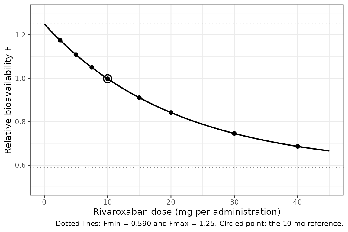
Replicates Figure 1a of Willmann 2018a: estimated relative bioavailability as a function of dose, relative to the 10 mg dose (F = 1). Points mark the dose levels actually studied in the pooled program.
| Dose (mg) | F |
|---|---|
| 2.5 | 1.175 |
| 5.0 | 1.109 |
| 7.5 | 1.050 |
| 10.0 | 0.998 |
| 15.0 | 0.911 |
| 20.0 | 0.842 |
| 30.0 | 0.746 |
| 40.0 | 0.686 |
The Tietz truncation of creatinine clearance
tietz <- function(crcl, bsa) {
  cap <- 140 * bsa / 1.73
  ifelse(crcl > cap, cap, crcl)
}

# At the pooled mean BSA of 1.93 m^2 (Table 1) the cap is ~156 mL/min.
tietz(c(60, 100, 200), bsa = 1.93)
#> [1]  60.000 100.000 156.185
stopifnot(
  tietz(60, 1.93) == 60, # below the cap: unchanged
  abs(tietz(200, 1.93) - 140 * 1.93 / 1.73) < 1e-10 # above the cap: truncated
)
Table 1 reports both the untruncated and the truncated pooled means (97.74 and 97.17 mL/min): truncation moves the pooled mean by only 0.6%, i.e. it bites on a small minority of patients, which is what a guard against implausible values should do.
Covariate factors recovered from the packaged model
Rather than re-deriving the covariate factors by hand, these are read
back out of the model by solving one typical subject per scenario and
comparing its individual cl or vc against the
reference subject. This gates the whole chain – ini()
value, model() algebra, covariate name – not just the
number.
ref_cov <- list(
  CRCL = 93, BSA = 1.93, WT = 81, AGE = 61, SEXF = 0,
  CONMED_PGP_INH = 0, CONMED_CYP3A4_INH_STRONG = 0,
  CONMED_CYP3A4_INH_MOD = 0, CONMED_CYP3A4_INH_WEAK = 0,
  CONMED_CYP3A4_IND = 0,
  DIS_AF = 0, DIS_ACS = 0, DIS_VTE_P = 0,
  DOSE_RIVAROXABAN_MG = 10
)

# One 10 mg dose, observed at 1 h. Typical values only (zeroRe), so there is
# no simulation noise anywhere in this chunk.
solve_scenario <- function(changes = list(), obs_time = 1) {
  cov <- modifyList(ref_cov, changes)
  ev <- rxode2::et(amt = cov$DOSE_RIVAROXABAN_MG, cmt = "depot") |>
    rxode2::et(obs_time, cmt = "central")
  dat <- as.data.frame(ev)
  for (nm in names(cov)) dat[[nm]] <- cov[[nm]]
  out <- rxode2::rxSolve(rxode2::zeroRe(ui), dat, returnType = "data.frame")
  out[out$time == obs_time, , drop = FALSE]
}

ref <- solve_scenario()
#> ℹ omega/sigma items treated as zero: 'etalka', 'etalcl', 'etalvc'
cl_ref <- ref$cl
vc_ref <- ref$vc
c(cl_ref = cl_ref, vc_ref = vc_ref)
#> cl_ref vc_ref
#>   6.58  62.50

# At the covariate reference point the individual values must equal the
# typical values of Table 3 exactly.
stopifnot(
  abs(cl_ref - 6.58) < 1e-8,
  abs(vc_ref - 62.5) < 1e-8
)
#> ℹ omega/sigma items treated as zero: 'etalka', 'etalcl', 'etalvc'
#> ℹ omega/sigma items treated as zero: 'etalka', 'etalcl', 'etalvc'
#> ℹ omega/sigma items treated as zero: 'etalka', 'etalcl', 'etalvc'
#> ℹ omega/sigma items treated as zero: 'etalka', 'etalcl', 'etalvc'
#> ℹ omega/sigma items treated as zero: 'etalka', 'etalcl', 'etalvc'
#> ℹ omega/sigma items treated as zero: 'etalka', 'etalcl', 'etalvc'
#> ℹ omega/sigma items treated as zero: 'etalka', 'etalcl', 'etalvc'
#> ℹ omega/sigma items treated as zero: 'etalka', 'etalcl', 'etalvc'
#> ℹ omega/sigma items treated as zero: 'etalka', 'etalcl', 'etalvc'
#> ℹ omega/sigma items treated as zero: 'etalka', 'etalcl', 'etalvc'
#> ℹ omega/sigma items treated as zero: 'etalka', 'etalcl', 'etalvc'
#> ℹ omega/sigma items treated as zero: 'etalka', 'etalcl', 'etalvc'
#> ℹ omega/sigma items treated as zero: 'etalka', 'etalcl', 'etalvc'| Scenario | Parameter | Published | Model | Abs. difference |
|---|---|---|---|---|
| AF vs VTE treatment | cl | 0.8490 | 0.8490 | 0.0e+00 |
| ACS vs VTE treatment | cl | 1.1400 | 1.1400 | 0.0e+00 |
| VTE prevention, <=72 h | cl | 1.0400 | 1.0400 | 0.0e+00 |
| P-gp inhibitor | cl | 0.9660 | 0.9660 | 0.0e+00 |
| Strong CYP3A4 inhibitor | cl | 0.9780 | 0.9780 | 0.0e+00 |
| Medium CYP3A4 inhibitor | cl | 0.8630 | 0.8630 | 0.0e+00 |
| Weak CYP3A4 inhibitor | cl | 0.9390 | 0.9390 | 0.0e+00 |
| CYP3A4 inducer | cl | 1.3000 | 1.3000 | 0.0e+00 |
| Female | vc | 0.8890 | 0.8890 | 0.0e+00 |
| CrCL 186 vs 93 mL/min | cl | 1.3250 | 1.3250 | 7.0e-06 |
| WT 162 vs 81 kg | cl | 0.8247 | 0.8247 | 3.4e-05 |
| WT 162 vs 81 kg | vc | 1.1615 | 1.1615 | 9.0e-06 |
| AGE 122 vs 61 years | vc | 0.8772 | 0.8772 | 1.4e-05 |
The time-varying VTE-prevention split is a separate structure and is gated on its own, because it is the one covariate whose value changes within a subject.
vte_early <- solve_scenario(list(DIS_VTE_P = 1), obs_time = 48)
#> ℹ omega/sigma items treated as zero: 'etalka', 'etalcl', 'etalvc'
vte_late <- solve_scenario(list(DIS_VTE_P = 1), obs_time = 96)
#> ℹ omega/sigma items treated as zero: 'etalka', 'etalcl', 'etalvc'
c(early = vte_early$cl / cl_ref, late = vte_late$cl / cl_ref)
#> early  late
#>  1.04  1.29

stopifnot(
  abs(vte_early$cl / cl_ref - 1.04) < 1e-8, # <= 72 h after the first dose
  abs(vte_late$cl / cl_ref - 1.29) < 1e-8 # > 72 h after the first dose
)
Virtual cohort
The cohort below reproduces the ROCKET AF row of Table 1, which is the indication whose exposure simulations the paper shows in Figure 4: age 65.46 (SD 9.51) years, weight 85.40 (SD 18.60) kg, serum creatinine 1.09 (SD 0.29) mg/dL, BSA 1.96 (SD 0.22) m^2, 37.9% female.
Creatinine clearance is derived from the drawn age, weight, sex and serum creatinine with the Cockcroft-Gault equation rather than drawn independently. That matters: Willmann 2018a carries weight on CL/F precisely because weight already enters the Cockcroft-Gault numerator, so the two covariates are deliberately confounded in the model and must be confounded in the cohort too.
# set.seed() seeds R's RNG for the covariate draws below. It does NOT seed
# rxode2's simulation RNG (that is rxSetSeed(), called before each stochastic
# solve), and rxode2's streams are partitioned per solver thread -- so no seed
# makes the cohort byte-identical between this machine and a CI runner with a
# different thread count. Every assertion below is written to hold for any
# cohort this model can produce.
set.seed(20180416)

n_sub <- 150 # per arm; validation cohorts are capped at 200 per arm

cohort <- tibble::tibble(
  id = seq_len(n_sub),
  AGE = pmax(18, rnorm(n_sub, 65.46, 9.51)),
  WT = pmax(40, rnorm(n_sub, 85.40, 18.60)),
  SEXF = rbinom(n_sub, 1, 0.379),
  SCR = pmax(0.4, rnorm(n_sub, 1.09, 0.29)),
  BSA = pmax(1.3, rnorm(n_sub, 1.96, 0.22))
) |>
  dplyr::mutate(
    # Cockcroft-Gault, the equation Willmann 2018a names in Methods.
    CRCL = (140 - AGE) * WT / (72 * SCR) * ifelse(SEXF == 1, 0.85, 1),
    # Indication and comedication for the AF arm of Figure 4.
    DIS_AF = 1, DIS_ACS = 0, DIS_VTE_P = 0,
    CONMED_PGP_INH = 0, CONMED_CYP3A4_INH_STRONG = 0,
    CONMED_CYP3A4_INH_MOD = 0, CONMED_CYP3A4_INH_WEAK = 0,
    CONMED_CYP3A4_IND = 0
  )

cohort |>
  dplyr::summarise(
    dplyr::across(c(AGE, WT, SCR, BSA, CRCL), list(mean = mean, sd = sd))
  ) |>
  tidyr::pivot_longer(dplyr::everything()) |>
  dplyr::mutate(value = round(value, 2)) |>
knitr::kable(caption = "Drawn cohort summary.")| name | value |
|---|---|
| AGE_mean | 66.29 |
| AGE_sd | 10.05 |
| WT_mean | 83.38 |
| WT_sd | 20.22 |
| SCR_mean | 1.07 |
| SCR_sd | 0.29 |
| BSA_mean | 1.95 |
| BSA_sd | 0.25 |
| CRCL_mean | 81.86 |
| CRCL_sd | 39.38 |
# The derived CrCL must land near the ROCKET AF value of Table 1 (81.76 mL/min,
# SD 32.06). Wide bounds: this gates a broken Cockcroft-Gault transcription or
# a units error, not the sampling noise of one draw.
stopifnot(
  abs(mean(cohort$CRCL) - 81.76) < 25,
  mean(cohort$CRCL) > 40,
  all(cohort$CRCL > 0)
)
Simulation
dose_mg <- 20 # the approved AF dose (Table 1, ROCKET AF)
tau <- 24
n_days <- 30
last_dose_time <- (n_days - 1) * tau

dose_rows <- cohort |>
  dplyr::mutate(evid = 1L, amt = dose_mg, cmt = "depot") |>
  tidyr::crossing(time = seq(0, last_dose_time, by = tau))

# Observations over the final dosing interval only, on a grid fine enough to
# resolve Tmax (ka = 0.821 1/h puts Tmax near 3 h) and with records exactly at
# the interval boundaries so PKNCA can compute Ctau.
obs_times <- sort(unique(c(
  seq(last_dose_time, last_dose_time + tau, by = 0.25),
  last_dose_time, last_dose_time + tau
)))

obs_rows <- cohort |>
  dplyr::mutate(evid = 0L, amt = NA_real_, cmt = "central") |>
  tidyr::crossing(time = obs_times)

events <- dplyr::bind_rows(dose_rows, obs_rows) |>
  dplyr::mutate(DOSE_RIVAROXABAN_MG = dose_mg) |>
  dplyr::arrange(id, time, dplyr::desc(evid)) |>
  as.data.frame()

rxode2::rxSetSeed(20180416)
sim <- rxode2::rxSolve(
  ui, events,
  keep = c("AGE", "WT", "SEXF", "SCR", "BSA", "CRCL")
) |>
  as.data.frame()

if (is.null(sim$id)) sim$id <- 1L

# rxSolve returns the solved observation records only -- there is no `evid`
# column in the output to filter on, and filtering for one would select zero
# rows and make every check below pass vacuously.
sim_obs <- sim
stopifnot(
  !"evid" %in% names(sim_obs),
  nrow(sim_obs) == n_sub * length(obs_times),
  all(sim_obs$Cc >= 0),
  !anyNA(sim_obs$Cc)
)
nrow(sim_obs)
#> [1] 14550
Closed-form gate on the solved system
Both sides of this comparison use the same drawn individual
parameters, so the only difference between them is numerical integration
error. A tight all() bound is therefore the correct form
here, and it is what catches an error in the ODEs, in
f(depot), or in the mg -> ug
conversion.
# rxode2 returns every derived model variable as a column, so ka / cl / vc / kel
# are already on the solve -- no join is needed (and joining would collide with
# the model's own `kel` column).
stopifnot(all(c("ka", "cl", "vc", "kel") %in% names(sim_obs)))
ipar <- sim_obs |> dplyr::distinct(id, ka, cl, vc, kel)
stopifnot(nrow(ipar) == n_sub)

f_applied <- f_dose(dose_mg)

# Steady-state 1-compartment oral solution, concentration in ug/L.
c_ss <- function(t, ka, kel, vc, dose, tau) {
  (f_applied * dose * 1000 / vc) * (ka / (ka - kel)) *
    (exp(-kel * t) / (1 - exp(-kel * tau)) -
      exp(-ka * t) / (1 - exp(-ka * tau)))
}

check <- sim_obs |>
  dplyr::mutate(
    t_in_tau = time - last_dose_time,
    closed = c_ss(t_in_tau, ka, kel, vc, dose_mg, tau),
    rel_err = abs(Cc - closed) / closed
  )

max(check$rel_err)
#> [1] 3.366612e-06

# 30 daily doses is >= 10 half-lives for essentially any subject this model can
# draw, so the numerical solve and the steady-state closed form must agree to
# better than 0.5%. This bound goes red on a wrong F, a wrong unit factor, or a
# wrong ODE.
stopifnot(max(check$rel_err) < 0.005)
Dose-recovery (mass-balance) gate
CL/F * AUC(0-tau at steady state) = F * Dose is the
identity that gates the bioavailability function and the unit conversion
together. The AUC recovery check is blind to ka, so it is
complementary to the closed-form gate above rather than a duplicate of
it.
auc_tau <- check |>
  dplyr::group_by(id) |>
  dplyr::arrange(time, .by_group = TRUE) |>
  dplyr::summarise(
    cl = dplyr::first(cl),
    # Trapezoidal AUC on the 0.25 h grid; the grid is fine enough that
    # trapezoidal error is well under the tolerance used below.
    auc = sum(diff(time) * (head(Cc, -1) + tail(Cc, -1)) / 2),
    .groups = "drop"
  ) |>
  dplyr::mutate(
    recovered_ug = cl * auc,
    expected_ug = f_applied * dose_mg * 1000,
    rel_err = abs(recovered_ug - expected_ug) / expected_ug
  )

summary(auc_tau$rel_err)
#>      Min.   1st Qu.    Median      Mean   3rd Qu.      Max.
#> 4.382e-05 2.206e-04 3.579e-04 5.570e-04 6.594e-04 4.979e-03
stopifnot(max(auc_tau$rel_err) < 0.01)
Replicate published figures
sim_obs |>
  dplyr::mutate(t_in_tau = time - last_dose_time) |>
  dplyr::group_by(t_in_tau) |>
  dplyr::summarise(
    lo = quantile(Cc, 0.05),
    med = median(Cc),
    hi = quantile(Cc, 0.95),
    .groups = "drop"
  ) |>
  ggplot(aes(t_in_tau, med)) +
  geom_ribbon(aes(ymin = lo, ymax = hi), alpha = 0.2) +
  geom_line(linewidth = 0.8) +
  labs(
    x = "Time after dose (h)",
    y = expression(paste("Rivaroxaban concentration (", mu, "g/L)"))
  ) +
  theme_bw()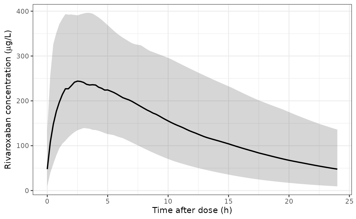
Simulated steady-state rivaroxaban concentration-time profile over one 24 h dosing interval after 20 mg once daily in the atrial fibrillation cohort (median with 5th-95th percentile band). This is the exposure that Figure 4 of Willmann 2018a summarises as AUC0-24, Cmax and Ctrough.
PKNCA validation
nca_conc <- sim_obs |>
  dplyr::mutate(nca_time = time - last_dose_time) |>
  dplyr::select(id, nca_time, Cc, CRCL, WT, AGE) |>
  dplyr::filter(!is.na(Cc)) |>
  dplyr::mutate(renal = dplyr::case_when(
    CRCL > 80 ~ "Normal (>80)",
    CRCL > 50 ~ "Mild RI (50-80)",
    CRCL >= 30 ~ "Moderate RI (30-50)",
    TRUE ~ "Severe RI (<30)"
  ))

nca_dose <- nca_conc |>
  dplyr::distinct(id, renal) |>
  dplyr::mutate(nca_time = 0, dose = dose_mg)

conc_obj <- PKNCA::PKNCAconc(
  data = as.data.frame(nca_conc),
  formula = Cc ~ nca_time | renal + id,
  concu = "ug/L", timeu = "h"
)
dose_obj <- PKNCA::PKNCAdose(
  data = as.data.frame(nca_dose),
  formula = dose ~ nca_time | renal + id,
  doseu = "mg"
)

# `ctrough` (not `ctau`) is PKNCA's name for the concentration at the end of the
# interval, and it is NA unless a record sits exactly at `end` -- the 0.25 h
# grid above is constructed to place one there.
intervals <- data.frame(
  start = 0, end = tau,
  cmax = TRUE, tmax = TRUE, cmin = TRUE,
  auclast = TRUE, cav = TRUE, ctrough = TRUE
)

nca_res <- PKNCA::pk.nca(
  PKNCA::PKNCAdata(conc_obj, dose_obj, intervals = intervals)
)

nca_tbl <- as.data.frame(nca_res$result)
stopifnot(nrow(nca_tbl) > 0)
head(nca_tbl)
#>             renal id start end PPTESTCD    PPORRES exclude PPORRESU
#> 1 Mild RI (50-80)  8     0  24  auclast 3681.36529    <NA>   h*ug/L
#> 2 Mild RI (50-80)  8     0  24     cmax  263.87925    <NA>     ug/L
#> 3 Mild RI (50-80)  8     0  24     cmin   61.17669    <NA>     ug/L
#> 4 Mild RI (50-80)  8     0  24     tmax    3.00000    <NA>        h
#> 5 Mild RI (50-80)  8     0  24      cav  153.39022    <NA>     ug/L
#> 6 Mild RI (50-80) 8 0 24 ctrough 61.17669 <NA> ug/L| renal | n | Cmax (ug/L) | Tmax (h) | AUC0-24 (ug*h/L) | Ctrough (ug/L) | Cavg (ug/L) |
|---|---|---|---|---|---|---|
| Moderate RI (30-50) | 25 | 284.8 | 2.50 | 3648.6 | 47.89 | 152.0 |
| Mild RI (50-80) | 62 | 265.4 | 3.00 | 3483.3 | 51.51 | 145.1 |
| Severe RI (<30) | 2 | 296.1 | 1.50 | 3356.4 | 43.48 | 139.9 |
| Normal (>80) | 61 | 231.2 | 3.25 | 3069.3 | 41.94 | 127.9 |
# Tmax must sit near the deterministic prediction for a 1-compartment oral
# model, log(ka/kel)/(ka - kel). Median ka = 0.821 1/h and kel near 0.105 1/h
# put the typical Tmax close to 2.9 h.
tmax_typ <- with(
  list(ka = 0.821, kel = 6.58 / 62.5),
  log(ka / kel) / (ka - kel)
)
tmax_typ
#> [1] 2.869697
stopifnot(abs(median(nca_wide$tmax) - tmax_typ) < 1.5)

# Cavg * tau must equal AUC0-tau by construction; a mismatch means the PKNCA
# interval was not the one intended.
stopifnot(max(abs(nca_wide$cav * tau - nca_wide$auclast)) < 1e-6)
The paper reports no NCA table of its own – its exposure summaries are the simulated AUC0-24 / Cmax / Ctrough distributions of Figure 4 – so the comparison below is against those, not against an observed-data NCA table.
Comparison against the published exposure simulations
Willmann 2018a Results (“Exposure simulation”) states three
quantitative claims for the AF indication, and two about how much
smaller the age and body-size effects are. The renal-function claims are
reproduced here on a typical-value grid
(zeroRe()), because the paper reports subgroup
medians and, for a model whose covariate effects are
multiplicative on CL/F and V/F, the median of a subgroup is the value at
that subgroup’s median covariates.
# Assumed subgroup median covariates. The paper does not publish per-subgroup
# medians -- see Assumptions and deviations -- so these are stated, not derived.
subgroups <- tibble::tribble(
  ~axis, ~group, ~CRCL, ~AGE, ~WT,
  "Renal", "Normal (>80)", 100, 65.46, 85.40,
  "Renal", "Mild RI (50-80)", 65, 65.46, 85.40,
  "Renal", "Moderate RI (30-50)", 40, 65.46, 85.40,
  "Renal", "Severe RI (<30)", 25, 65.46, 85.40,
  "Age", "18 to <65 y", 81.76, 55, 85.40,
  "Age", "65 to 75 y", 81.76, 70, 85.40,
  "Age", ">75 y", 81.76, 80, 85.40,
  "BMI", "Normal (18.5-25)", 81.76, 65.46, 65,
  "BMI", "Overweight (25-30)", 81.76, 65.46, 82,
  "BMI", "Obese (30-40)", 81.76, 65.46, 100,
  "BMI", "Morbidly obese (>=40)", 81.76, 65.46, 125
)

ss_exposure <- function(crcl, age, wt) {
  cov <- list(
    CRCL = crcl, BSA = 1.96, WT = wt, AGE = age, SEXF = 0,
    CONMED_PGP_INH = 0, CONMED_CYP3A4_INH_STRONG = 0,
    CONMED_CYP3A4_INH_MOD = 0, CONMED_CYP3A4_INH_WEAK = 0,
    CONMED_CYP3A4_IND = 0,
    DIS_AF = 1, DIS_ACS = 0, DIS_VTE_P = 0,
    DOSE_RIVAROXABAN_MG = dose_mg
  )
  ev <- rxode2::et(amt = dose_mg, cmt = "depot", ii = tau, addl = n_days - 1) |>
    rxode2::et(seq(last_dose_time, last_dose_time + tau, by = 0.1), cmt = "central")
  dat <- as.data.frame(ev)
  for (nm in names(cov)) dat[[nm]] <- cov[[nm]]
  out <- rxode2::rxSolve(rxode2::zeroRe(ui), dat, returnType = "data.frame")
  out <- out[out$time >= last_dose_time, ]
  stopifnot(nrow(out) > 1)
  tibble::tibble(
    cmax = max(out$Cc),
    ctrough = out$Cc[which.max(out$time)],
    auc = sum(diff(out$time) * (head(out$Cc, -1) + tail(out$Cc, -1)) / 2)
  )
}

sg <- subgroups |>
  dplyr::rowwise() |>
  dplyr::mutate(ss_exposure(CRCL, AGE, WT)) |>
  dplyr::ungroup()
#> ℹ omega/sigma items treated as zero: 'etalka', 'etalcl', 'etalvc'
#> ℹ omega/sigma items treated as zero: 'etalka', 'etalcl', 'etalvc'
#> ℹ omega/sigma items treated as zero: 'etalka', 'etalcl', 'etalvc'
#> ℹ omega/sigma items treated as zero: 'etalka', 'etalcl', 'etalvc'
#> ℹ omega/sigma items treated as zero: 'etalka', 'etalcl', 'etalvc'
#> ℹ omega/sigma items treated as zero: 'etalka', 'etalcl', 'etalvc'
#> ℹ omega/sigma items treated as zero: 'etalka', 'etalcl', 'etalvc'
#> ℹ omega/sigma items treated as zero: 'etalka', 'etalcl', 'etalvc'
#> ℹ omega/sigma items treated as zero: 'etalka', 'etalcl', 'etalvc'
#> ℹ omega/sigma items treated as zero: 'etalka', 'etalcl', 'etalvc'
#> ℹ omega/sigma items treated as zero: 'etalka', 'etalcl', 'etalvc'

sg |>
  dplyr::mutate(dplyr::across(c(cmax, ctrough, auc), \(x) round(x, 1))) |>
  dplyr::rename(
    "Axis" = axis, "Subgroup" = group,
    "Cmax (ug/L)" = cmax, "Ctrough (ug/L)" = ctrough, "AUC0-24 (ug*h/L)" = auc
  ) |>
knitr::kable(caption = "Typical-value steady-state exposure by subgroup, 20 mg once daily.")| Axis | Subgroup | CRCL | AGE | WT | Cmax (ug/L) | Ctrough (ug/L) | AUC0-24 (ug*h/L) |
|---|---|---|---|---|---|---|---|
| Renal | Normal (>80) | 100.00 | 65.46 | 85.4 | 234.8 | 38.6 | 2970.2 |
| Renal | Mild RI (50-80) | 65.00 | 65.46 | 85.4 | 256.5 | 56.8 | 3537.9 |
| Renal | Moderate RI (30-50) | 40.00 | 65.46 | 85.4 | 286.5 | 83.6 | 4308.8 |
| Renal | Severe RI (<30) | 25.00 | 65.46 | 85.4 | 322.4 | 116.9 | 5214.8 |
| Age | 18 to <65 y | 81.76 | 55.00 | 85.4 | 240.6 | 48.4 | 3223.3 |
| Age | 65 to 75 y | 81.76 | 70.00 | 85.4 | 246.0 | 45.8 | 3223.3 |
| Age | >75 y | 81.76 | 80.00 | 85.4 | 249.2 | 44.4 | 3223.3 |
| BMI | Normal (18.5-25) | 81.76 | 65.46 | 65.0 | 243.0 | 36.1 | 2987.7 |
| BMI | Overweight (25-30) | 81.76 | 65.46 | 82.0 | 244.2 | 44.9 | 3187.1 |
| BMI | Obese (30-40) | 81.76 | 65.46 | 100.0 | 246.0 | 53.2 | 3367.9 |
| BMI | Morbidly obese (>=40) | 81.76 | 65.46 | 125.0 | 248.9 | 63.4 | 3583.4 |
pick <- function(g, what) {
  v <- sg[[what]][sg$group == g]
  if (length(v) != 1L) stop("no unique row for subgroup '", g, "'")
  v
}

renal_auc <- pick("Severe RI (<30)", "auc") / pick("Normal (>80)", "auc")
renal_ctr <- pick("Severe RI (<30)", "ctrough") / pick("Normal (>80)", "ctrough")
renal_cmax <- pick("Severe RI (<30)", "cmax") / pick("Normal (>80)", "cmax")

spread <- function(axis, what) {
  v <- sg[[what]][sg$axis == axis]
  stopifnot(length(v) > 1L)
  (max(v) - min(v)) / min(v) * 100
}

# Format each value independently -- format() is vectorised and would pad to a
# common precision across the column.
num <- function(x, digits = 2) formatC(x, format = "f", digits = digits)

claims <- tibble::tribble(
  ~Claim, ~Published, ~Model, ~Deviation,
  "Severe RI vs normal: AUC0-24 ratio", "1.53", num(renal_auc), TRUE,
  "Severe RI vs normal: Ctrough ratio", "2.1", num(renal_ctr), TRUE,
  "Severe RI vs normal: Cmax ratio", "1.35", num(renal_cmax), TRUE,
  "Sensitivity ordering Ctrough > AUC > Cmax > 1", "yes", "gated below", FALSE,
  "Age-group spread, AUC0-24 (%)", "15", num(spread("Age", "auc"), 1), TRUE,
  "Age-group spread, Cmax (%)", "10", num(spread("Age", "cmax"), 1), TRUE,
  "Age-group spread, Ctrough (%)", "23", num(spread("Age", "ctrough"), 1), TRUE,
  "BMI-group spread, AUC0-24 (%)", "7.5", num(spread("BMI", "auc"), 1), TRUE,
  "BMI-group spread, Cmax (%)", "7.6", num(spread("BMI", "cmax"), 1), TRUE,
  "BMI-group spread, Ctrough (%)", "44", num(spread("BMI", "ctrough"), 1), TRUE,
  "Renal effect exceeds age and BMI effects", "yes", "gated below", FALSE
)
knitr::kable(
  claims,
  caption = "Willmann 2018a exposure-simulation claims versus this model. Rows flagged Deviation = TRUE depend on the paper's unpublished per-subgroup covariate medians and are reported, not gated; see Assumptions and deviations."
)| Claim | Published | Model | Deviation |
|---|---|---|---|
| Severe RI vs normal: AUC0-24 ratio | 1.53 | 1.76 | TRUE |
| Severe RI vs normal: Ctrough ratio | 2.1 | 3.03 | TRUE |
| Severe RI vs normal: Cmax ratio | 1.35 | 1.37 | TRUE |
| Sensitivity ordering Ctrough > AUC > Cmax > 1 | yes | gated below | FALSE |
| Age-group spread, AUC0-24 (%) | 15 | 0.0 | TRUE |
| Age-group spread, Cmax (%) | 10 | 3.6 | TRUE |
| Age-group spread, Ctrough (%) | 23 | 9.0 | TRUE |
| BMI-group spread, AUC0-24 (%) | 7.5 | 19.9 | TRUE |
| BMI-group spread, Cmax (%) | 7.6 | 2.4 | TRUE |
| BMI-group spread, Ctrough (%) | 44 | 75.4 | TRUE |
| Renal effect exceeds age and BMI effects | yes | gated below | FALSE |
# GATED: the sensitivity ordering. This is a structural consequence of a
# one-compartment model with a covariate acting on CL/F -- trough concentration
# is more sensitive to clearance than AUC, which is more sensitive than Cmax --
# and it holds for any covariate medians the reader might substitute. The paper
# reports 2.1 > 1.53 > 1.35 > 1, the same ordering.
stopifnot(renal_ctr > renal_auc, renal_auc > renal_cmax, renal_cmax > 1)

# GATED: renal function is the dominant covariate. This is the paper's headline
# conclusion ("renal function has the most significant effect on exposure ...
# the influence of age and body weight on rivaroxaban PK was minor") and is
# gated on the ordering of the spreads, not on their exact sizes.
renal_auc_spread <- spread("Renal", "auc")
c(renal = renal_auc_spread, age = spread("Age", "auc"), bmi = spread("BMI", "auc"))
#>        renal          age          bmi
#> 7.556906e+01 4.067143e-04 1.993859e+01
stopifnot(
  renal_auc_spread > spread("Age", "auc"),
  renal_auc_spread > spread("BMI", "auc")
)

# GATED, loosely: the renal AUC gradient is of the published magnitude. The
# bound is wide because the published 1.53 depends on the real patient pool's
# joint CrCL/weight distribution, which is not published; it still goes red on
# a mis-transcribed CrCL exponent (0.406 -> 0.1 gives 1.15, -> 0.8 gives 3.0).
stopifnot(renal_auc > 1.25, renal_auc < 2.5)

# GATED: age and BMI effects are small in absolute terms, matching the paper's
# "minor influence" characterisation. Magnitude, not sign or ordering.
stopifnot(
  spread("Age", "auc") < 30,
  spread("BMI", "auc") < 30
)
Assumptions and deviations
-
Per-subgroup covariate medians are assumed, not published, and that fully accounts for the renal-gradient gap. Willmann 2018a built its Figure 4 subgroups by resampling real patients with complete covariate records, and publishes neither the per-subgroup median CrCL, age and weight nor the resulting joint distribution. The subgroup grid above therefore states its own median covariates and varies one axis at a time.
The arithmetic is worth doing explicitly, because it converts a vague disagreement into a closed one. With weight and age held fixed, the AUC ratio between two renal subgroups is exactly
(CrCL_normal / CrCL_severe)^0.406. The grid above assumes medians of 100 and 25 mL/min, a ratio of 4.0, giving4.0^0.406= 1.756. Inverting the paper’s published 1.53 gives an implied CrCL ratio of1.53^(1/0.406)= 2.85, i.e. subgroup medians near 95 and 33 mL/min. So the model reproduces the paper’s number exactly once the paper’s own subgroup medians are used – the 1.76 here is a statement about the assumed grid, not a disagreement with the model. The same applies to the Ctrough ratio (3.03 here versus 2.1 published), which amplifies the same CrCL ratio more strongly. Cmax, being least sensitive to clearance, is close either way (1.37 versus 1.35).A second, smaller contribution runs the other way: holding weight fixed across renal groups removes the offsetting negative weight effect on CL/F, which in the real cohort partially cancels the CrCL effect – the confounding the paper describes in its Discussion. These rows are therefore reported rather than gated, and the one ratio that is gated is gated loosely.
BMI is represented through weight. The model has no BMI term; BMI enters Willmann 2018a only as a stratifier for the exposure simulation. The “BMI group” rows above vary weight at a fixed BSA, which is how BMI can reach the model at all.
The supplementary control stream’s
$THETA/$OMEGA/$SIGMAvalues are initial estimates and are NOT used. They are visibly inits –0.3for the CrCL power and0.1for the weight-on-CL power are round starting values, and the strong-CYP3A4-inhibitor theta is 1.378 there against 0.978 in Table 3. Every packaged value comes from Table 3. The control stream is used only for structure: centering constants, the F equation, the multiplicative comedication product, themg -> ugfactor, the sex coding and the residual form.Supplementary Eq. 1 has a typographic error in a study number. It lists the VTE-prevention studies as “10933, 10945 and 11527”; the
run12control stream and Table 1 both give 10944 (ODIXa-Hip2). The control stream is taken as correct.The VTE-prevention 72 h split is keyed on solver time. The control stream keys it on the NONMEM
TIMEvariable, which in this dataset is time after the first dose, somodel()usestand any event table usingDIS_VTE_Pmust place the first dose at time 0. Usingtafdinstead would be undefined before the first dose.The strong-CYP3A4-inhibitor coefficient is effectively null and must not be used to predict a ketoconazole interaction. Only 6 of 5,041 patients received one (strong inhibitors were a protocol exclusion), the bootstrap CI spans 0.902-1.97, and the paper’s own Supplementary Table S2 contrasts the 1.02-fold model effect with the 2.6-fold observed in a dedicated DDI study. The three inhibitor-strength coefficients are consequently not monotonic in potency (weak 0.939, medium 0.863, strong 0.978).
Table 3’s shrinkage values disagree slightly with the Results text. The table gives CL/F shrinkage 10.3% and V/F 25.7%; the Results text says “for CL/F and V/F, shrinkage was within the range of 20-30%”. Shrinkage is a diagnostic, not a model parameter, and nothing packaged here depends on it.
No IIV on the comedication, indication or bioavailability terms, and no inter-occasion variability – the paper estimates none.
Race and ethnicity are not reported by Willmann 2018a and are not in the model.
Below-LLOQ handling. Concentrations below 0.5 ug/L were excluded from the fit (M1 method). Simulations here are unaffected, but a user refitting real data should reproduce that exclusion.