Omega-3 PUFA (Wang 2024)
Source:vignettes/articles/Wang_2024_omega3PUFA.Rmd
Wang_2024_omega3PUFA.RmdModel and source
- Citation: Wang L, Huang X, Sun M, Zheng T, Zheng L, Lin X, Ruan J, Lin F. New light on omega-3 polyunsaturated fatty acids and diabetes debate: a population pharmacokinetic-pharmacodynamic modelling and intake threshold study. Nutr Diabetes. 2024;14(1):8. doi:10.1038/s41387-024-00262-w
- Description: One-compartment population PK model with first-order oral absorption for omega-3 polyunsaturated fatty acids (PUFA) in community-dwelling adults with type 2 diabetes, with an HDL-cholesterol power covariate on Ka, V and CL, coupled to a direct-effect inhibitory Imax model for glycosylated hemoglobin (HbA1c) (Wang 2024)
- Article: Nutr Diabetes. 2024;14(1):8 (open access; PMC10912742)
Wang 2024 is, to the authors’ knowledge, the first population pharmacokinetic-pharmacodynamic (PPK-PD) analysis of a nutrient rather than a drug. Habitual dietary omega-3 polyunsaturated fatty acid (PUFA) intake, measured by food-frequency questionnaire, is treated as the dose; plasma omega-3 PUFA measured by ELISA is the PK observation; and glycosylated hemoglobin (HbA1c) is the PD observation. The analysis was used to propose an intake threshold for patients with type 2 diabetes.
Population
161 community-dwelling adults with type 2 diabetes were recruited from the East Street and South Street communities of Fuzhou, Fujian Province, China, during 2020-2021 in a two-centre prospective study (ChiCTR2000036210). Participants were aged 43-85 years (mean 67.2), 97 of 161 (60.2%) female, weighed 39-102 kg (mean 63.5) with a BMI of 16.0-43.8 kg/m^2. Baseline HbA1c was 6.31 +/- 1.91 % (median 5.7, range 2-14.1) and plasma omega-3 PUFA 0.0319 +/- 0.0091 g/L (median 0.0299, range 0.0107-0.0508). Habitual omega-3 PUFA intake ranged 0.036-6.426 g/day (mean 1.14, median 0.774). HDL cholesterol, the only covariate retained in the final model, was 1.38 +/- 0.38 mmol/L (median 1.28, range 0.77-2.49). All demographics are from Wang 2024 Table 1. A separate group of 49 patients with type 2 diabetes served as the external validation set. Race/ethnicity was not reported.
The same information is available programmatically via
readModelDb("Wang_2024_omega3PUFA")()$population.
Structural model
Wang 2024 describes the disposition model as “the two-compartment
model with first-order elimination”. The final model, however, estimates
only Ka, V and CL (Table 2) –
there is no intercompartmental clearance and no peripheral volume
anywhere in the paper. The authors are counting the absorption
(depot) compartment as the second compartment; the
disposition itself is one-compartment. Two independent checks confirm
this reading:
- The paper’s own derived half-life, “~43.86 h … deduced from the
pharmacokinetic formula”, equals
log(2) * V / CL = log(2) * 26.151 / 0.411 =44.10 h. A genuinely two-compartment model would have a terminal half-life governed by the beta phase, which cannot be computed fromVandCLalone. - The steady-state exposure implied by
CLalone reproduces the paper’s published dose-threshold simulations (see “Replicating Figure 2” below).
The packaged model is therefore depot ->
central with first-order absorption and first-order
elimination, coupled to a direct-effect inhibitory Imax model for
HbA1c.
Source trace
Per-parameter origins are recorded as in-file comments next to each
ini() entry in
inst/modeldb/specificDrugs/Wang_2024_omega3PUFA.R. They are
collected here for review.
| Equation / parameter | Value | Source location |
|---|---|---|
lka (Ka) |
1.175 1/h | Table 2, “Final model” column; printed Ka equation, p. 3 |
lvc (V/F) |
26.151 L | Table 2, “Final model” column; printed V equation, p. 3 |
lcl (CL/F) |
0.411 L/h | Table 2, “Final model” column; printed CL equation, p. 3 |
e_hdlc_ka |
0.007 | Printed final-model equation, p. 3:
Ka = 1.175 * (HDL/1.38)^0.007
|
e_hdlc_vc |
-0.535 | Printed final-model equation, p. 3:
V = 26.151 * (HDL/1.38)^(-0.535)
|
e_hdlc_cl |
0.285 | Printed final-model equation, p. 3:
CL = 0.411 * (HDL/1.38)^0.285
|
| HDL-C reference value | 1.38 mmol/L | Table 1 (cohort mean HDL); appears as the divisor in all three printed equations |
le0 (E0) |
5.641 % | Table 2, “Final model” column |
lec50 (IC50) |
0.090 g/L | Table 2, “Final model” column |
limax (Imax) |
0.597 %-points | Table 2, “Final model” column |
propSd |
0.354 | Table 2, PK block, “sigma” row, “Final model” column |
propSd_hba1c |
0.354 | Table 2, PD block, “sigma” row, “Final model” column |
d/dt(depot), d/dt(central)
|
n/a | Implied by the Ka / V / CL parameterisation, p. 3 |
hba1c effect equation |
n/a | Not printed; form resolved against Figure 2 and the Results dose claims (see below) |
All eta terms |
fixed at 0 |
exp(etaKa), exp(etaV),
exp(etaCL), exp(etaE0),
exp(etaIC50), exp(etaImax) appear in the
printed equations, p. 3; no omega is reported anywhere |
Note that the parenthesised numbers in Table 2’s “Final model (CV%)”
column are relative standard errors of the estimates,
not inter-individual variability: the residual-error
term sigma also carries one, and a residual-error parameter
has no IIV.
Virtual cohort
The original observed data are not publicly available. The cohort below reproduces the HDL-C distribution of Wang 2024 Table 1 (mean 1.38, SD 0.38, median 1.28, range 0.77-2.49 mmol/L). Mean exceeds median, so a lognormal matched to the reported mean and SD is used, truncated to the observed range.
set.seed(20240308)
n_subj <- 161L

# Lognormal moment-matched to mean 1.38, SD 0.38, truncated to [0.77, 2.49]
hdlc_sd_log <- sqrt(log(1 + (0.38 / 1.38)^2))
hdlc_mu_log <- log(1.38) - hdlc_sd_log^2 / 2
hdlc <- rlnorm(n_subj, hdlc_mu_log, hdlc_sd_log)
hdlc <- pmin(pmax(hdlc, 0.77), 2.49)

cohort <- tibble(id = seq_len(n_subj), HDLC = hdlc)

tibble(
  Statistic = c("Mean", "SD", "Median", "Minimum", "Maximum"),
  Simulated = c(mean(hdlc), sd(hdlc), median(hdlc), min(hdlc), max(hdlc)),
  `Wang 2024 Table 1` = c(1.38, 0.38, 1.28, 0.77, 2.49)
) |>
  mutate(across(where(is.numeric), \(x) round(x, 3))) |>
knitr::kable(caption = "Virtual-cohort HDL-C (mmol/L) vs. Wang 2024 Table 1.")| Statistic | Simulated | Wang 2024 Table 1 |
|---|---|---|
| Mean | 1.368 | 1.38 |
| SD | 0.370 | 0.38 |
| Median | 1.309 | 1.28 |
| Minimum | 0.770 | 0.77 |
| Maximum | 2.490 | 2.49 |
Simulation
Observation records are written on the Cc endpoint.
Cc and hba1c are both declared endpoints of
this model (each has its own ~ residual line), so rxode2
allocates their observation slots as part of the model definition; a
single set of observation rows returns both model variables as output
columns.
mod <- readModelDb("Wang_2024_omega3PUFA")

# Three HDL-C strata spanning the observed range, single 1 g oral dose.
hdl_strata <- tibble(
  id        = 1:3,
  HDLC      = c(0.77, 1.38, 2.49),
  hdl_group = c("HDL-C 0.77 mmol/L (minimum)",
                "HDL-C 1.38 mmol/L (cohort mean)",
                "HDL-C 2.49 mmol/L (maximum)")
)

ev_sd <- hdl_strata |>
  tidyr::crossing(time = c(0, sort(unique(c(seq(0.25, 12, by = 0.25),
                                            seq(12, 480, by = 2)))))) |>
  mutate(amt = NA_real_, evid = 0L, cmt = "Cc") |>
  bind_rows(
    hdl_strata |> mutate(time = 0, amt = 1, evid = 1L, cmt = "depot")
  ) |>
  arrange(id, time, desc(evid)) |>
  as.data.frame()

sim_sd <- rxode2::rxSolve(mod, ev_sd, keep = "hdl_group",
                          returnType = "data.frame")
#> ℹ parameter labels from comments will be replaced by 'label()'
#> ℹ omega/sigma items treated as zero: 'etalka', 'etalvc', 'etalcl', 'etale0', 'etalec50', 'etalimax'
#> Warning: multi-subject simulation without without 'omega'

ggplot(sim_sd, aes(time, Cc, colour = hdl_group)) +
  geom_line(linewidth = 0.7) +
  scale_x_continuous(limits = c(0, 336)) +
  labs(x = "Time (h)", y = "Plasma omega-3 PUFA (g/L)", colour = NULL,
       title = "Single 1 g oral dose across the observed HDL-C range",
       caption = paste("Wang 2024 final model. Higher HDL-C raises CL/F",
                       "(exponent +0.285) and lowers V/F (exponent -0.535).")) +
  theme(legend.position = "bottom")
#> Warning: Removed 216 rows containing missing values or values outside the scale range
#> (`geom_line()`).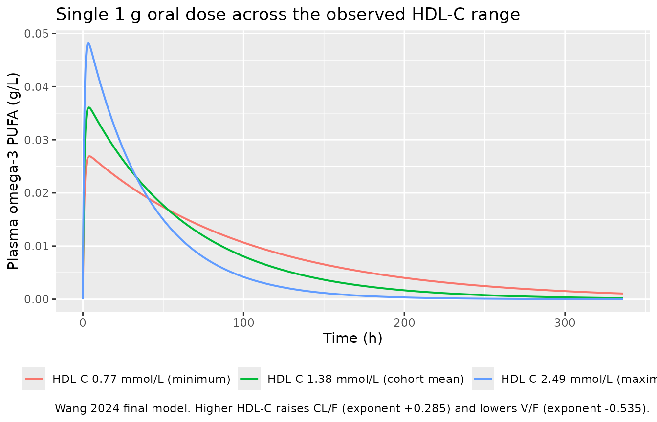
PKNCA validation
sim_nca <- sim_sd |>
  dplyr::filter(!is.na(Cc)) |>
  dplyr::select(id, time, Cc, hdl_group)

# Guarantee a time = 0 record per subject; pre-dose Cc is 0 for an oral dose.
sim_nca <- dplyr::bind_rows(
  sim_nca,
  sim_nca |> dplyr::distinct(id, hdl_group) |> dplyr::mutate(time = 0, Cc = 0)
) |>
  dplyr::distinct(id, hdl_group, time, .keep_all = TRUE) |>
  dplyr::arrange(id, hdl_group, time)

conc_obj <- PKNCA::PKNCAconc(sim_nca, Cc ~ time | hdl_group + id)

dose_df <- ev_sd |>
  dplyr::filter(evid == 1) |>
  dplyr::select(id, time, amt, hdl_group)

dose_obj <- PKNCA::PKNCAdose(dose_df, amt ~ time | hdl_group + id)

intervals <- data.frame(
  start = 0, end = Inf,
  cmax = TRUE, tmax = TRUE, aucinf.obs = TRUE, half.life = TRUE
)

nca_res <- PKNCA::pk.nca(PKNCA::PKNCAdata(conc_obj, dose_obj,
                                          intervals = intervals))
Comparison against published values
Wang 2024 reports exactly one NCA-type quantity: a half-life of “~43.86 h”, stated for the typical patient. It is compared below against the simulated half-life in each HDL-C stratum; only the cohort-mean stratum has a published reference, so the other two rows carry no reference value by design.
published <- tibble::tribble(
  ~hdl_group,                        ~half.life,
  "HDL-C 0.77 mmol/L (minimum)",     NA_real_,
  "HDL-C 1.38 mmol/L (cohort mean)", 43.86,
  "HDL-C 2.49 mmol/L (maximum)",     NA_real_
)

cmp <- nlmixr2lib::ncaComparisonTable(
  simulated     = nca_res,
  reference     = published,
  by            = "hdl_group",
  units         = c(half.life = "h"),
  tolerance_pct = 20
)

cmp |>
  dplyr::rename("HDL-C stratum" = hdl_group) |>
  knitr::kable(
    caption = paste("Simulated half-life vs. the ~43.86 h reported by",
                    "Wang 2024 (Discussion, p. 6).",
                    "* differs from reference by >20%."),
    align = c("l", "l", "r", "r", "r")
)| NCA parameter | HDL-C stratum | Reference | Simulated | % diff |
|---|---|---|---|---|
| t½ (h) | HDL-C 0.77 mmol/L (minimum) | — | 71.2 | — |
| t½ (h) | HDL-C 1.38 mmol/L (cohort mean) | 43.9 | 44.1 | +0.6% |
| t½ (h) | HDL-C 2.49 mmol/L (maximum) | — | 27.2 | — |
Implementation identity checks
For a linear one-compartment model with first-order absorption,
AUC(0-inf) and Tmax follow analytically from
F, Dose, CL, Ka and
kel. These are not independent published values – they are
derived from the same Table 2 estimates – so they check that the
packaged ODE system implements those estimates correctly rather than
validating the estimates themselves.
th   <- rxode2::rxode(mod)$theta
#> ℹ parameter labels from comments will be replaced by 'label()'
ka_i <- exp(th[["lka"]]) * (hdl_strata$HDLC / 1.38)^th[["e_hdlc_ka"]]
vc_i <- exp(th[["lvc"]]) * (hdl_strata$HDLC / 1.38)^th[["e_hdlc_vc"]]
cl_i <- exp(th[["lcl"]]) * (hdl_strata$HDLC / 1.38)^th[["e_hdlc_cl"]]
kel_i <- cl_i / vc_i

nca_wide <- as.data.frame(nca_res) |>
  dplyr::select(hdl_group, PPTESTCD, PPORRES) |>
  tidyr::pivot_wider(names_from = PPTESTCD, values_from = PPORRES)

tibble(
  hdl_group          = hdl_strata$hdl_group,
  `AUCinf simulated` = nca_wide$aucinf.obs[match(hdl_strata$hdl_group,
                                                 nca_wide$hdl_group)],
  `AUCinf = Dose/CL` = 1 / cl_i,
  `Tmax simulated`   = nca_wide$tmax[match(hdl_strata$hdl_group,
                                           nca_wide$hdl_group)],
  `Tmax analytic`    = log(ka_i / kel_i) / (ka_i - kel_i)
) |>
  mutate(across(where(is.numeric), \(x) round(x, 3))) |>
  dplyr::rename("HDL-C stratum" = hdl_group) |>
  knitr::kable(
    caption = paste("Analytic identities for a linear one-compartment model.",
                    "AUCinf in g*h/L, Tmax in h."),
    align = c("l", "r", "r", "r", "r")
)| HDL-C stratum | AUCinf simulated | AUCinf = Dose/CL | Tmax simulated | Tmax analytic |
|---|---|---|---|---|
| HDL-C 0.77 mmol/L (minimum) | 2.873 | 2.873 | 4.25 | 4.126 |
| HDL-C 1.38 mmol/L (cohort mean) | 2.433 | 2.433 | 3.75 | 3.722 |
| HDL-C 2.49 mmol/L (maximum) | 2.056 | 2.056 | 3.25 | 3.322 |
Resolving the HbA1c effect equation
Wang 2024 prints the three individual-parameter equations for
E0, IC50 and Imax, and defines
them in words (“E0 is the baseline effect, IC50 is the drug
concentration corresponding to the 50% maximum inhibitory effect, and
Imax is the maximum inhibitory effect”), but never prints the effect
equation itself. Two readings are standard:
-
fractional,
HbA1c = E0 * (1 - Imax * Cc / (IC50 + Cc)), in whichImaxis a dimensionless fraction of baseline; and -
additive,
HbA1c = E0 - Imax * Cc / (IC50 + Cc), in whichImaxis an absolute maximal reduction in HbA1c percentage points.
The paper’s own simulation outputs settle the question. Figure 2
plots target attainment against daily intake for four HbA1c targets, and
at a dose of zero the drug term vanishes under either reading –
so the zero-dose intercepts identify the population spread on
E0 alone, independently of the effect form. Reading the
four intercepts off the published panel and inverting a lognormal gives
a consistent spread:
E0 <- exp(rxode2::rxode(mod)$theta[["le0"]])
#> ℹ parameter labels from comments will be replaced by 'label()'

# Digitised from the published Figure 2 panel at dose = 0 g/day.
fig2_zero <- tibble(
  target  = c(6.5, 7.0, 7.5, 8.0),
  attain  = c(0.830, 0.930, 0.975, 0.997)
) |>
  mutate(`implied omega_E0` = log(target / E0) / qnorm(attain))

omega_e0 <- mean(fig2_zero$`implied omega_E0`)

fig2_zero |>
  mutate(across(where(is.numeric), \(x) round(x, 4))) |>
  dplyr::rename("HbA1c target (%)" = target,
                "Attainment at 0 g/day" = attain) |>
  knitr::kable(caption = paste0(
    "Zero-dose intercepts of Wang 2024 Figure 2 inverted through a lognormal ",
"E0. Mean implied omega_E0 = ", round(omega_e0, 4), "."))| HbA1c target (%) | Attainment at 0 g/day | implied omega_E0 |
|---|---|---|
| 6.5 | 0.830 | 0.1485 |
| 7.0 | 0.930 | 0.1463 |
| 7.5 | 0.975 | 0.1453 |
| 8.0 | 0.997 | 0.1271 |
Four independent targets imply essentially the same spread
(0.127-0.149), which supports the lognormal-E0 reading.
Holding omega_E0 fixed at that zero-dose value, the
entire dose-response of Figure 2 is then an out-of-sample
prediction of the packaged PK-PD model. The two candidate effect forms
give very different answers.
th <- rxode2::rxode(mod)$theta
#> ℹ parameter labels from comments will be replaced by 'label()'
imax_v <- exp(th[["limax"]]); ec50_v <- exp(th[["lec50"]])
cl_ref <- exp(th[["lcl"]])

# Average steady-state concentration for a once-daily intake, F = 1.
css <- function(dose) dose / (cl_ref * 24)
drop <- function(dose) imax_v * css(dose) / (ec50_v + css(dose))

typ_frac <- function(dose) E0 * (1 - imax_v * css(dose) / (ec50_v + css(dose)))
typ_add  <- function(dose) E0 -      imax_v * css(dose) / (ec50_v + css(dose))

attain <- function(typfun, dose, target, omega) {
  pnorm(log(target / typfun(dose)) / omega)
}

doses <- c(0, 0.4, 0.8, 1.2, 1.6)
bind_rows(
  tidyr::crossing(dose = doses, target = c(6.5, 7.0, 7.5, 8.0)) |>
    mutate(form = "additive",
           attainment = 100 * attain(typ_add, dose, target, omega_e0)),
  tidyr::crossing(dose = doses, target = c(6.5, 7.0, 7.5, 8.0)) |>
    mutate(form = "fractional",
           attainment = 100 * attain(typ_frac, dose, target, omega_e0))
) |>
  mutate(attainment = round(attainment, 1)) |>
  tidyr::pivot_wider(names_from = target, values_from = attainment,
                     names_prefix = "HbA1c <= ") |>
  dplyr::rename("Effect form" = form, "Intake (g/day)" = dose) |>
  knitr::kable(caption = paste(
    "Predicted target attainment (%) under each candidate effect form, using",
    "only the zero-dose omega_E0. Published Figure 2 reads approximately",
"83 / 93 / 97.5 / 99.7 at 0 g/day and 90.5 / 96 / 99 / 100 at 1.6 g/day."))| Intake (g/day) | Effect form | HbA1c <= 6.5 | HbA1c <= 7 | HbA1c <= 7.5 | HbA1c <= 8 |
|---|---|---|---|---|---|
| 0.0 | additive | 84.1 | 93.6 | 97.8 | 99.3 |
| 0.4 | additive | 89.2 | 96.1 | 98.8 | 99.7 |
| 0.8 | additive | 91.3 | 97.0 | 99.1 | 99.8 |
| 1.2 | additive | 92.5 | 97.5 | 99.3 | 99.8 |
| 1.6 | additive | 93.3 | 97.8 | 99.4 | 99.8 |
| 0.0 | fractional | 84.1 | 93.6 | 97.8 | 99.3 |
| 0.4 | fractional | 99.3 | 99.9 | 100.0 | 100.0 |
| 0.8 | fractional | 100.0 | 100.0 | 100.0 | 100.0 |
| 1.2 | fractional | 100.0 | 100.0 | 100.0 | 100.0 |
| 1.6 | fractional | 100.0 | 100.0 | 100.0 | 100.0 |
The fractional form drives attainment to 100% at every target for any intake at or above 0.4 g/day – inconsistent with a figure whose 6.5% curve never exceeds about 91%. The additive form tracks all four published curves. It is also the only form consistent with the two numeric claims in the Results:
tibble(
  Claim = c("0.4 g/day, HbA1c 7.0%", "1.3 g/day, HbA1c 6.5%"),
  `Wang 2024` = c("> 95%", "90.08%"),
  `Additive form` = sprintf("%.1f%%", 100 * c(
    attain(typ_add, 0.4, 7.0, omega_e0), attain(typ_add, 1.3, 6.5, omega_e0))),
  `Fractional form` = sprintf("%.1f%%", 100 * c(
    attain(typ_frac, 0.4, 7.0, omega_e0), attain(typ_frac, 1.3, 6.5, omega_e0)))
) |>
  knitr::kable(caption = paste(
    "Wang 2024 Results dose claims vs. each candidate effect form.",
"omega_E0 comes only from the zero-dose intercepts of Figure 2."))| Claim | Wang 2024 | Additive form | Fractional form |
|---|---|---|---|
| 0.4 g/day, HbA1c 7.0% | > 95% | 96.1% | 99.9% |
| 1.3 g/day, HbA1c 6.5% | 90.08% | 92.7% | 100.0% |
The packaged model therefore implements
hba1c <- e0 - imax * Cc / (ec50 + Cc), with
Imax = 0.597 interpreted as an absolute maximal reduction
of 0.597 HbA1c percentage points.
Replicating Figure 2
The replication below runs the packaged model over the virtual cohort
at each intake level, dosing once daily to steady state, and averages
Cc over the final dosing interval – HbA1c integrates
glycaemia over roughly three months, so the average steady-state
concentration is the appropriate driver. Target attainment is then
evaluated by integrating the lognormal E0 spread
analytically for each subject, which removes Monte-Carlo noise in the
dimension that matters (published and predicted attainments differ by
only a few percentage points).
dose_levels <- c(0, 0.2, 0.4, 0.8, 1.2, 1.6)

# 30 daily doses reaches steady state (half-life ~44 h); observe over day 30.
# NOTE: the carried dose-level column must NOT be called `dose` -- rxode2's
# etTrans() consumes a column of that name, and `keep = "dose"` then fails with
# "Cannot keep missing columns".
build_arm <- function(dose, id_offset) {
  subj <- cohort |> mutate(id = id + id_offset, intake_g = dose)
  obs <- subj |>
    tidyr::crossing(time = seq(24 * 29, 24 * 30, by = 1)) |>
    mutate(amt = NA_real_, evid = 0L, cmt = "Cc")
  dos <- subj |>
    tidyr::crossing(time = seq(0, 24 * 29, by = 24)) |>
    mutate(amt = dose, evid = 1L, cmt = "depot")
  bind_rows(obs, dos) |> arrange(id, time, desc(evid))
}

ev_ss <- do.call(
  bind_rows,
  lapply(seq_along(dose_levels), function(i) {
    build_arm(dose_levels[i], (i - 1L) * 1000L)
  })
) |>
  as.data.frame()

stopifnot(!anyDuplicated(unique(ev_ss[, c("id", "time", "evid")])))

sim_ss <- rxode2::rxSolve(mod, ev_ss, keep = c("intake_g"),
                          returnType = "data.frame")
#> ℹ omega/sigma items treated as zero: 'etalka', 'etalvc', 'etalcl', 'etale0', 'etalec50', 'etalimax'
#> Warning: multi-subject simulation without without 'omega'
stopifnot("intake_g" %in% names(sim_ss))

# Average Cc over the final dosing interval, per subject and intake level.
css_subj <- sim_ss |>
  dplyr::filter(!is.na(Cc)) |>
  group_by(id, intake_g) |>
  summarise(css = mean(Cc), .groups = "drop")

# rxSolve can silently drop subjects; assert the full grid came back.
stopifnot(nrow(css_subj) == n_subj * length(dose_levels))

# Attainment: P(E0 * exp(eta) - drop <= target), eta ~ N(0, omega_E0^2).
attainment <- css_subj |>
  mutate(drop = imax_v * css / (ec50_v + css)) |>
  tidyr::crossing(target = c(6.5, 7.0, 7.5, 8.0)) |>
  mutate(p = pnorm(log((target + drop) / E0) / omega_e0)) |>
  group_by(intake_g, target) |>
  summarise(attainment = 100 * mean(p), .groups = "drop")

published_fig2 <- tibble::tribble(
  ~intake_g, ~target, ~attainment,
  0.0, 6.5, 83.0,  0.0, 7.0, 93.0,  0.0, 7.5, 97.5,  0.0, 8.0, 99.7,
  0.4, 6.5, 88.5,  0.4, 7.0, 95.5,  0.4, 7.5, 98.5,  0.4, 8.0, 99.9,
  1.6, 6.5, 90.5,  1.6, 7.0, 96.0,  1.6, 7.5, 99.0,  1.6, 8.0, 99.9
)

ggplot(attainment, aes(intake_g, attainment,
                       colour = factor(target), group = factor(target))) +
  geom_line(linewidth = 0.7) +
  geom_point(size = 1.6) +
  geom_point(data = published_fig2, shape = 4, size = 3, stroke = 1) +
  scale_y_continuous(limits = c(80, 100)) +
  labs(x = "Omega-3 PUFA intake (g/day)",
       y = "Target attainment of HbA1c (%)",
       colour = "HbA1c target (%)",
       title = "Replicates Figure 2 of Wang 2024",
       caption = paste("Lines: packaged model over the virtual cohort.",
                       "Crosses: values digitised from the published Figure 2.")) +
  theme(legend.position = "bottom")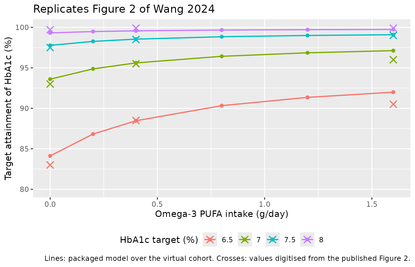
attainment |>
  left_join(published_fig2 |> dplyr::rename(published = attainment),
            by = c("intake_g", "target")) |>
  mutate(attainment = round(attainment, 1),
         difference = round(attainment - published, 1)) |>
  dplyr::rename("Intake (g/day)" = intake_g, "HbA1c target (%)" = target,
                "Simulated (%)" = attainment, "Wang 2024 Figure 2 (%)" = published,
                "Difference (pp)" = difference) |>
  knitr::kable(
    caption = paste("Simulated vs. digitised Figure 2 target attainment.",
                    "Blank reference cells are intake levels not read off",
                    "the published panel."),
    align = c("r", "r", "r", "r", "r")
)| Intake (g/day) | HbA1c target (%) | Simulated (%) | Wang 2024 Figure 2 (%) | Difference (pp) |
|---|---|---|---|---|
| 0.0 | 6.5 | 84.1 | 83.0 | 1.1 |
| 0.0 | 7.0 | 93.6 | 93.0 | 0.6 |
| 0.0 | 7.5 | 97.8 | 97.5 | 0.3 |
| 0.0 | 8.0 | 99.3 | 99.7 | -0.4 |
| 0.2 | 6.5 | 86.8 | NA | NA |
| 0.2 | 7.0 | 94.9 | NA | NA |
| 0.2 | 7.5 | 98.3 | NA | NA |
| 0.2 | 8.0 | 99.5 | NA | NA |
| 0.4 | 6.5 | 88.5 | 88.5 | 0.0 |
| 0.4 | 7.0 | 95.6 | 95.5 | 0.1 |
| 0.4 | 7.5 | 98.5 | 98.5 | 0.0 |
| 0.4 | 8.0 | 99.6 | 99.9 | -0.3 |
| 0.8 | 6.5 | 90.3 | NA | NA |
| 0.8 | 7.0 | 96.4 | NA | NA |
| 0.8 | 7.5 | 98.8 | NA | NA |
| 0.8 | 8.0 | 99.7 | NA | NA |
| 1.2 | 6.5 | 91.4 | NA | NA |
| 1.2 | 7.0 | 96.9 | NA | NA |
| 1.2 | 7.5 | 99.0 | NA | NA |
| 1.2 | 8.0 | 99.7 | NA | NA |
| 1.6 | 6.5 | 92.0 | 90.5 | 1.5 |
| 1.6 | 7.0 | 97.1 | 96.0 | 1.1 |
| 1.6 | 7.5 | 99.1 | 99.0 | 0.1 |
| 1.6 | 8.0 | 99.7 | 99.9 | -0.2 |
Agreement is within about 2 percentage points at every intake level
and target that could be read off the published panel. Because
omega_E0 was fitted only to the zero-dose intercepts, every
non-zero-dose point is an out-of-sample prediction of the packaged PK
and PD parameters together.
HDL-C covariate effect
hdl_grid <- tibble(HDLC = seq(0.77, 2.49, length.out = 60)) |>
  mutate(
    `CL/F (L/h)` = exp(th[["lcl"]]) * (HDLC / 1.38)^th[["e_hdlc_cl"]],
    `V/F (L)`    = exp(th[["lvc"]]) * (HDLC / 1.38)^th[["e_hdlc_vc"]],
    `Half-life (h)` = log(2) * `V/F (L)` / `CL/F (L/h)`
  ) |>
  tidyr::pivot_longer(-HDLC, names_to = "parameter", values_to = "value")

ggplot(hdl_grid, aes(HDLC, value)) +
  geom_line(linewidth = 0.7) +
  geom_vline(xintercept = 1.38, linetype = "dashed", colour = "grey50") +
  facet_wrap(~parameter, scales = "free_y") +
  labs(x = "HDL cholesterol (mmol/L)", y = NULL,
       title = "HDL-C effect over the observed range",
       caption = paste("Dashed line: the reference HDL-C of 1.38 mmol/L.",
                       "Wang 2024 printed final-model equations, p. 3."))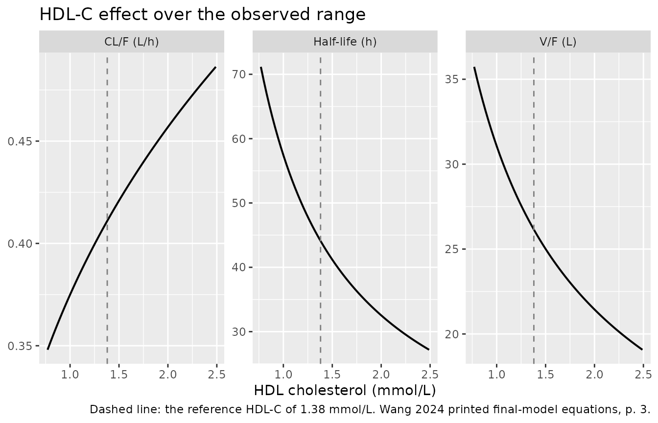
Across the observed HDL-C range the model predicts a 39.7% span in
CL/F and a substantially wider span in half-life, because
V/F moves in the opposite direction (exponent -0.535) to
CL/F (exponent +0.285).
Assumptions and deviations
“Two-compartment” nomenclature. Wang 2024 calls the disposition model two-compartment, but reports only
Ka,VandCL, and its own derived half-life islog(2) * V / CL. The packaged model is one-compartment with a first-order absorption depot, as the equations require. See “Structural model”.The
exp(eta)terms are typeset inside the covariate exponent. The published equations render as, for example,CL = 0.411 * (HDL/1.38)^(0.285 * exp(etaCL)), with the whole product in the superscript. Taken literally this is degenerate: any subject with the reference HDL-C of 1.38 mmol/L would have1^x = 1and therefore no inter-individual variability at all. The packaged model uses the standard Phoenix NLME formtheta * (cov / ref)^theta_cov * exp(eta), treating the superscript scope as a typesetting artefact.Sign of the
V/Fexponent. TheVexponent is negative (-0.535) in the published equation. Text-extraction tools drop the superscript minus sign; the value was confirmed against the rendered PDF page.Direction of the HDL-C effect on clearance. The Discussion states that “in patients with lower HDL, the clearance of omega-3 PUFA was accelerated”, which implies a negative CL exponent. The printed equation has a positive exponent (+0.285), so lower HDL-C gives lower CL/F and higher exposure. The equation is used, per the standing policy that a printed equation takes precedence over narrative text. This conflict is unresolved in the source and reviewers should be aware of it.
The HbA1c effect equation is not printed in the paper. The additive form
HbA1c = E0 - Imax * Cc / (IC50 + Cc)was selected because it reproduces Figure 2 and both quoted dose claims, while the fractional alternative misses them by more than 12 percentage points. The full derivation is in “Resolving the HbA1c effect equation”. No parameter value was altered to achieve the agreement.No inter-individual variability is reported. The printed equations contain
exp(etaKa),exp(etaV),exp(etaCL),exp(etaE0),exp(etaIC50)andexp(etaImax), but Wang 2024 never reports a single omega – the parenthesised numbers in Table 2 are relative standard errors, since the residual-error termsigmaalso carries one. All six etas are therefore declared and fixed at zero in the model file, preserving the published structure without inventing variances. Theomega_E0 =0.142 used in this vignette is not part of the packaged model: it is derived here by digitising the zero-dose intercepts of Figure 2 and is used only to reproduce that figure.Residual error form. Table 2 reports a bare
sigmaof 0.354 for each sub-model with no error-model statement. An additive interpretation is dimensionally impossible for the PK observation (0.354 against plasma levels around 0.03 g/L), so both are encoded as proportional. Note also that Table 2’s PDsigmarow carries a bootstrap median of 1.615 with a 2.5th-97.5th percentile range of 0.354-0.354, which does not bracket its own median; this row appears to be mis-transcribed in the source.Bioavailability fixed at 1.
Fis not reported.F = 1is supported independently: the steady-state exposureDose / (CL * 24)computed withF = 1reproduces the published Figure 2 and both dose-threshold claims. Note that this is not consistent with the observed data in Table 1 – a median habitual intake of 0.774 g/day implies a steady-state level of 0.0785 g/L against an observed median plasma level of 0.0299 g/L, a factor of about 2.6. The published simulations behave as thoughF = 1, soF = 1is what the packaged model implements.Table 2 versus the printed PD equations. The printed PD equations quote
E0 = 5.5796,IC50 = 0.089andImax = 0.615, which are the bootstrap medians from Table 2, not the final-model estimates (5.641, 0.090, 0.597). The printed PK equations, by contrast, quote the final-model estimates exactly. The packaged model uses the “Final model” column of Table 2 throughout, for internal consistency. The two sets differ by less than 3% and neither choice changes any conclusion in this vignette.Covariate distribution. HDL-C is drawn from a lognormal moment-matched to the Table 1 mean and SD and truncated to the observed range; the joint distribution of covariates was not published. Race/ethnicity was not reported and is not modelled.
Dose interpretation. The “dose” is habitual dietary omega-3 PUFA intake quantified by food-frequency questionnaire, not an administered dose. Intake was treated as a once-daily oral input in the steady-state simulations, matching the paper’s “daily intake” framing.