Norepinephrine (Oualha 2014)
Source:vignettes/articles/Oualha_2014_norepinephrine.Rmd
Oualha_2014_norepinephrine.RmdModel and source
- Citation: Oualha M, Treluyer JM, Lesage F, de Saint Blanquat L, Dupic L, Hubert P, Spreux-Varoquaux O, Urien S (2014). Population pharmacokinetics and haemodynamic effects of norepinephrine in hypotensive critically ill children. British Journal of Clinical Pharmacology 78(4):886-897. doi:10.1111/bcp.12412.
- Article: https://doi.org/10.1111/bcp.12412
- Source: paper text + Tables 1, 2, 3 + Figure 8 (dosing simulations).
The published model is a paediatric population PK/PD analysis of continuous IV norepinephrine in hypotensive critically ill children. It combines:
- a one-compartment open PK sub-model with first-order elimination and
an endogenous zero-order norepinephrine production rate
q0(Methods PK/PD modelling), - allometric weight scaling on CL and
q0with the exponent FIXED to 3/4 (Table 2; Results paragraph 1 of “Norepinephrine pharmacokinetics”), - a circulating-volume formula Vc = 0.08 * BW (Methods, cited from Linderkamp via the V_circ rule; Table 2 footnote),
- an Emax PD sub-model on mean arterial pressure (MAP) with a power-of-PCA effect on basal MAP0 and a categorical organ-dysfunction-count effect on the maximal drug-induced MAP increase dMAP (Eq. for MAP; Table 3).
Population
Thirty-eight critically ill children were enrolled at a single tertiary paediatric ICU (Hopital Necker Enfants-Malades, Paris, January 2011 - December 2012; Oualha 2014 Table 1) after presenting with systemic arterial hypotension. Body weight ranged from 2 to 85 kg (median 6.7 kg) and age from 0 to 182 months (median 7.6 months); the cohort included 7 premature neonates (GA 32-36 weeks). Aetiologies of hypotension were septic shock (n=16), non-traumatic cerebral injury (n=6), heavy sedation (n=8), and severe congenital diaphragmatic defect (n=8). Norepinephrine was infused continuously at 0.05-2 ug/kg/min (median 0.5) for a median of 1.5 days (range 1-13). Fourteen of 38 children (37%) had more than 3 concurrent organ dysfunctions; 17 (45%) died during ICU stay.
The same information is available programmatically:
mod_meta <- rxode2::rxode2(readModelDb("Oualha_2014_norepinephrine"))$meta
#> ℹ parameter labels from comments will be replaced by 'label()'
mod_meta$population$species
#> [1] "human"
mod_meta$population$n_subjects
#> [1] 38
mod_meta$population$disease_state
#> [1] "Critically ill children with systemic arterial hypotension (septic shock n=16, non-traumatic cerebral injury n=6, heavy sedation n=8, severe congenital diaphragmatic defect n=8) requiring continuous IV norepinephrine for haemodynamic support."
Source trace
The per-parameter origin is recorded as an in-file comment next to
each ini() entry in
inst/modeldb/specificDrugs/Oualha_2014_norepinephrine.R.
The table below collects them in one place for review.
| Symbol | Value | Source location |
|---|---|---|
| theta_CL (typical unit clearance, L/h/kg^0.75) | 6.6 | Table 2 |
| theta_BW exponent (CL) | 0.75 (FIXED) | Table 2; Results “Norepinephrine pharmacokinetics” |
| theta_q0 (typical unit endogenous production, ug/h/kg^0.75) | 3.12 | Table 2 |
| theta_BW exponent (q0) | 0.75 (FIXED) | Table 2 |
| V_circ = 0.08 * BW (L) | 0.08 L/kg | Methods; Table 2 footnote |
| omega(CL), omega(q0) | 0.6, 1.1 (sqrt of omega^2) | Table 2 |
| propSd (NorEp concentration) | 0.25 | Table 2 |
| MAP0 (mmHg) | 34 | Table 3 |
| theta_PCA on MAP0 | 0.166 | Table 3 |
| dMAP (org dysfn <=3) | 32 mmHg | Table 3 |
| dMAP (org dysfn >=4) | 12 mmHg | Table 3 |
| EC50_MAP (ug/L) | 4.11 | Table 3 |
| omega(MAP0), omega(dMAP) | 0.17, 0.3 | Table 3 |
| propSd_MAP | 0.14 | Table 3 |
| dA/dt = q0 + Rate - CL * Cc | n/a | Methods PK/PD modelling |
| V = 0.08 * BW | n/a | Methods; Table 2 footnote |
| MAP = MAP0 + dMAP * Cc / (Cc + EC50) | n/a | Methods PK/PD modelling, Eq. for MAP |
| MAP0_i = MAP0 * (PCA / 9)^theta_PCA | n/a | Results “Norepinephrine pharmacodynamics” |
Virtual cohort
Original observed data are not publicly available. The cohort below mirrors the five illustrative scenarios used in Figure 8 of Oualha 2014 (children spanning the cohort weight / age range), with each scenario simulated under two organ-dysfunction strata (orgf_high = 0 for ORG_FAIL_COUNT <= 3, orgf_high = 1 for ORG_FAIL_COUNT >= 4) and a grid of infusion rates from 0 to 2 ug/kg/min. Postmenstrual age values assume term-newborn gestational age 40 weeks (9 months) plus postnatal age in months, matching the typical-subject definitions used in the paper’s Figure 8 simulation.
set.seed(20140506)  # paper acceptance date

horizon_h <- 1  # NorEp t1/2 is ~1 min for a 10 kg child, so 1 h far exceeds 5 * t1/2

scenarios <- tibble::tribble(
  ~scenario,         ~wt,  ~age_mo, ~page_mo,
  "3 kg neonate",    3,    0.462,   0.462 + 9,    # term-newborn PCA reference
  "10 kg infant",    10,   12,      12 + 9,
  "20 kg child",     20,   72,      72 + 9,
  "40 kg child",     40,   144,     144 + 9,
  "70 kg adult-size",70,   300,     300 + 9
)

dose_grid <- c(0, 0.05, 0.1, 0.2, 0.5, 1.0, 1.5, 2.0)  # ug/kg/min, paper range

cohort <- tidyr::expand_grid(
  scenarios,
  org_fail_high = c(0L, 1L),
  dose_ug_kg_min = dose_grid
) |>
  dplyr::mutate(
    treatment      = sprintf("%s | orgf=%s | %.2f ug/kg/min",
                             scenario,
                             ifelse(org_fail_high == 1L, ">=4", "<=3"),
                             dose_ug_kg_min),
    rate_ug_per_h  = dose_ug_kg_min * wt * 60,
    amt_total      = rate_ug_per_h * horizon_h * 2,  # > horizon -> infusion runs to end
    ORG_FAIL_COUNT = ifelse(org_fail_high == 1L, 4L, 0L),
    id             = dplyr::row_number()
  )

obs_grid_h <- c(0, seq(1/60, horizon_h, by = 1/60))  # 1-minute grid

build_events <- function(.cohort, obs_grid) {
  dose_rows <- .cohort |>
    dplyr::filter(rate_ug_per_h > 0) |>
    dplyr::transmute(
      id, time = 0, evid = 1L,
      amt = amt_total, rate = rate_ug_per_h, cmt = "central",
      treatment, WT = wt, PAGE = page_mo, ORG_FAIL_COUNT
    )
  obs_rows <- tidyr::expand_grid(
    .cohort |> dplyr::select(id, treatment, WT = wt, PAGE = page_mo, ORG_FAIL_COUNT),
    time = obs_grid
  ) |>
    dplyr::mutate(evid = 0L, amt = NA_real_, rate = NA_real_, cmt = "Cc")
  dplyr::bind_rows(dose_rows, obs_rows) |>
    dplyr::arrange(id, time, dplyr::desc(evid))
}

events <- build_events(cohort, obs_grid_h)
stopifnot(!anyDuplicated(unique(events[, c("id", "time", "evid")])))
Simulation
mod <- readModelDb("Oualha_2014_norepinephrine")
mod_typ <- mod |> rxode2::zeroRe()
#> ℹ parameter labels from comments will be replaced by 'label()'

sim_typ <- rxode2::rxSolve(
  mod_typ, events,
  keep = c("treatment", "WT", "PAGE", "ORG_FAIL_COUNT")
) |>
  as.data.frame() |>
  dplyr::left_join(
    cohort |> dplyr::select(id, scenario, org_fail_high, dose_ug_kg_min),
    by = "id"
  )
#> ℹ omega/sigma items treated as zero: 'etalcl', 'etalq0', 'etalmap0', 'etaldmap'
#> Warning: multi-subject simulation without without 'omega'
Replicate published figures
Figure 8 – Steady-state Cc and MAP vs infusion rate
Figure 8 of Oualha 2014 plots typical-value norepinephrine concentration (linear in infusion rate) and the haemodynamic response (curvilinear, Emax-shaped on MAP) versus infusion rate for the five reference WT / age scenarios, separately for the two organ-dysfunction strata.
We reach the steady-state value at the end of the 1-hour horizon (well past five times the longest scenario half-life of ~1.5 min in a 70-kg subject).
ss_typ <- sim_typ |>
  dplyr::group_by(id, scenario, org_fail_high, dose_ug_kg_min) |>
  dplyr::filter(time == max(time)) |>
  dplyr::ungroup() |>
  dplyr::mutate(
    orgf_label = ifelse(org_fail_high == 1L,
                        "ORG_FAIL_COUNT >= 4",
                        "ORG_FAIL_COUNT <= 3"),
    scenario   = factor(
      scenario,
      levels = c("3 kg neonate", "10 kg infant", "20 kg child",
                 "40 kg child", "70 kg adult-size")
    )
  )
ggplot(ss_typ, aes(dose_ug_kg_min, Cc, colour = scenario)) +
  geom_line() + geom_point() +
  facet_wrap(~orgf_label) +
  labs(x = "Norepinephrine infusion rate (ug/kg/min)",
       y = "Steady-state Cc (ug/L)",
       title = "Figure 8a -- typical-value Cc vs infusion rate",
       caption = paste("Replicates the concentration panel of Figure 8 in",
                       "Oualha 2014. Cc is linear in infusion rate per",
                       "Cc_ss = (q0 + Rate) / CL."))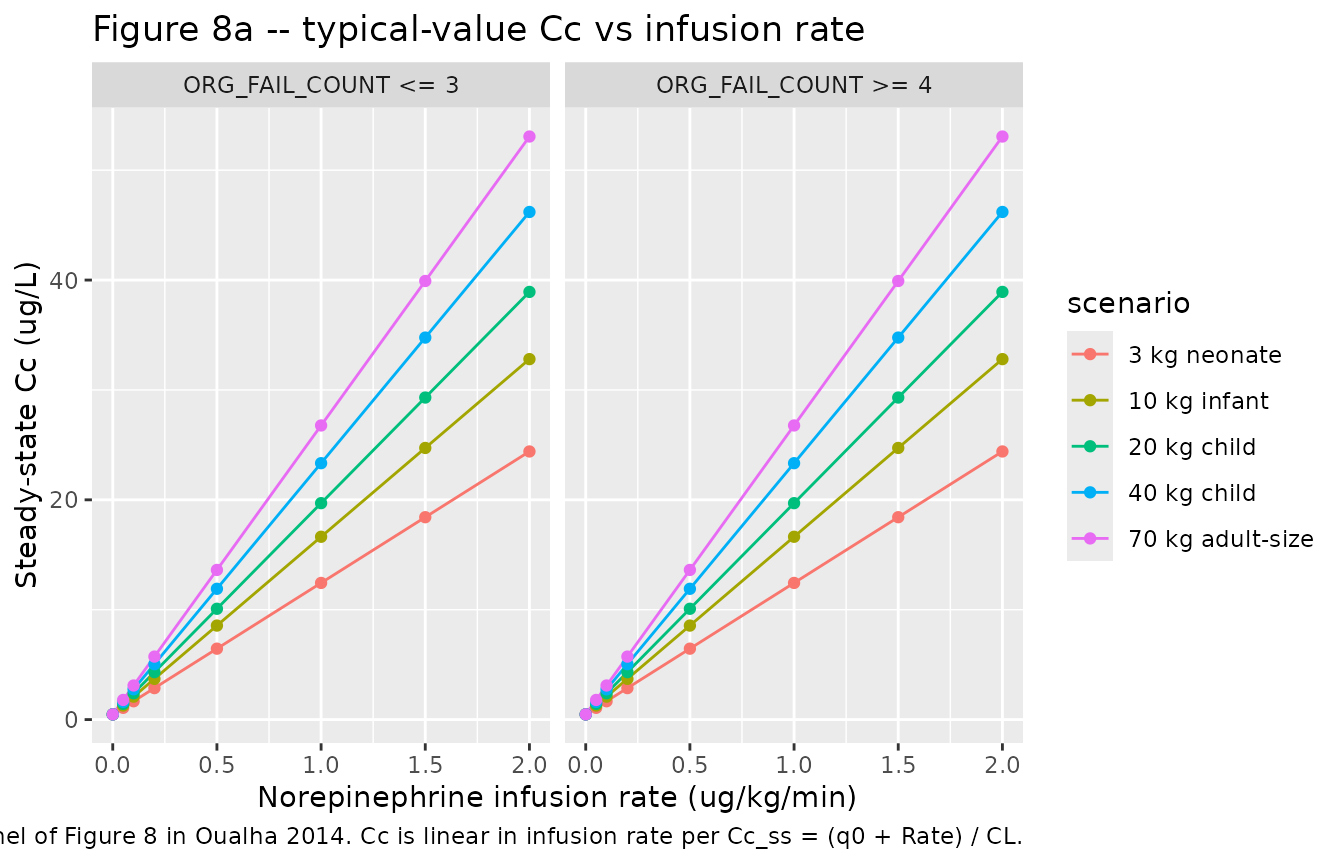
ggplot(ss_typ, aes(dose_ug_kg_min, MAP, colour = scenario)) +
  geom_line() + geom_point() +
  facet_wrap(~orgf_label) +
  labs(x = "Norepinephrine infusion rate (ug/kg/min)",
       y = "Steady-state MAP (mmHg)",
       title = "Figure 8b -- typical-value MAP vs infusion rate",
       caption = paste("Replicates the MAP panel of Figure 8 in Oualha",
                       "2014. The curvilinear shape reflects the Cc-MAP",
                       "Emax response. The lower asymptote at infusion",
                       "rate 0 is the age-dependent basal MAP0; the upper",
                       "asymptote is map0 + dmap, where dmap = 32 for",
                       "orgf_high = 0 and 12 for orgf_high = 1."))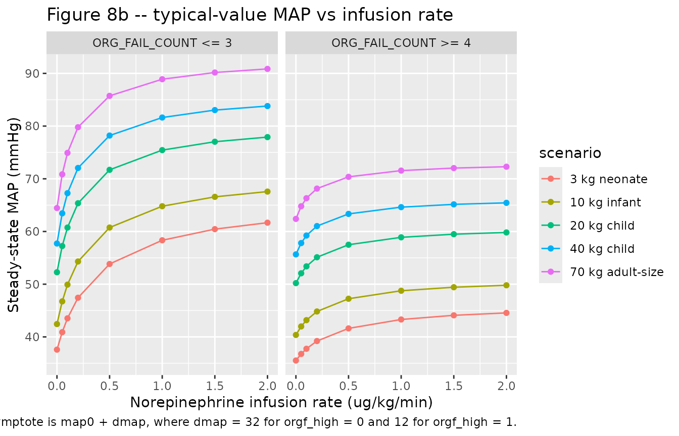
The MAP panel reproduces the paper’s central clinical finding: in children with more than three organ dysfunctions, the maximum achievable MAP increase from norepinephrine is markedly smaller (12 mmHg vs 32 mmHg), which manifests as a much shallower MAP-vs-rate response.
PKNCA validation
Because norepinephrine is infused continuously and reaches steady state within ~5 plasma half-lives (~5 min for a 10 kg child), classical single-dose NCA is not the natural validation tool. Instead we compute PKNCA steady-state summaries (Cmax, Cmin, Cav over the last 30 minutes of the 1-hour observation window) and compare against the paper’s reported plasma norepinephrine concentration during infusion: median 3.75 ug/L (range 0.88-46) per Results paragraph 1 of “Norepinephrine pharmacokinetics”.
sim_pk <- sim_typ |>
  dplyr::filter(!is.na(Cc)) |>
  dplyr::select(id, time, Cc, treatment)

# Guarantee a time = 0 row per (id, treatment) -- the Cc at t=0 is the
# endogenous-only baseline q0/cl produced by the model's central(0)
# initial condition, which the simulation already includes; the
# bind_rows pattern below is the defensive idiom from pknca-recipes.md.
sim_pk <- dplyr::bind_rows(
  sim_pk,
  sim_pk |>
    dplyr::distinct(id, treatment) |>
    dplyr::filter(!id %in% sim_pk$id[sim_pk$time == 0]) |>
    dplyr::mutate(time = 0, Cc = NA_real_)
) |>
  dplyr::distinct(id, treatment, time, .keep_all = TRUE) |>
  dplyr::arrange(id, treatment, time)

dose_df <- events |>
  dplyr::filter(evid == 1) |>
  dplyr::select(id, time, amt, treatment)

conc_obj <- PKNCA::PKNCAconc(
  sim_pk, Cc ~ time | treatment + id,
  concu = "ug/L", timeu = "h"
)
dose_obj <- PKNCA::PKNCAdose(
  dose_df, amt ~ time | treatment + id,
  doseu = "ug"
)

# Steady-state interval over the last 30 minutes of the 1-hour run.
intervals <- data.frame(
  start = 0.5, end = 1.0,
  cmax  = TRUE, cmin = TRUE, cav  = TRUE
)

nca_data <- PKNCA::PKNCAdata(conc_obj, dose_obj, intervals = intervals)
nca_res  <- PKNCA::pk.nca(nca_data)
nca_tbl  <- as.data.frame(nca_res$result)
Comparison against published cohort-wide median
Restricting to the cohort-median scenario (10 kg infant, ORG_FAIL_COUNT <=3, median infusion rate 0.5 ug/kg/min), the simulated steady-state norepinephrine concentration is:
median_scenario <- ss_typ |>
  dplyr::filter(scenario == "10 kg infant",
                org_fail_high == 0,
                dplyr::near(dose_ug_kg_min, 0.5))

simulated <- tibble::tibble(
  source = "Oualha 2014 model, 10 kg infant, ORG_FAIL_COUNT <= 3, 0.5 ug/kg/min",
  Cc_steady_state_ug_per_L = round(median_scenario$Cc, 2),
  MAP_steady_state_mmHg    = round(median_scenario$MAP, 1)
)

published <- tibble::tibble(
  source = paste("Oualha 2014 Table 1 / Results paragraph 1 of",
                 "Norepinephrine pharmacokinetics (cohort median during",
                 "infusion)"),
  Cc_observed_median_ug_per_L = 3.75,
  Cc_observed_range_ug_per_L  = "0.88 to 46"
)

published_map <- tibble::tibble(
  source = paste("Oualha 2014 Results paragraph 1 of Norepinephrine",
                 "pharmacodynamics (cohort median MAP under infusion)"),
  MAP_observed_median_mmHg = 50,
  MAP_observed_range_mmHg  = "25 to 92"
)

knitr::kable(simulated,
             caption = paste("Simulated typical-value steady-state Cc and",
"MAP for the cohort-median scenario."))| source | Cc_steady_state_ug_per_L | MAP_steady_state_mmHg |
|---|---|---|
| Oualha 2014 model, 10 kg infant, ORG_FAIL_COUNT <= 3, 0.5 ug/kg/min | 8.56 | 60.8 |
knitr::kable(published,
caption = "Published cohort-wide median NorEp concentration during infusion.")| source | Cc_observed_median_ug_per_L | Cc_observed_range_ug_per_L |
|---|---|---|
| Oualha 2014 Table 1 / Results paragraph 1 of Norepinephrine pharmacokinetics (cohort median during infusion) | 3.75 | 0.88 to 46 |
knitr::kable(published_map,
caption = "Published cohort-wide median MAP under infusion.")| source | MAP_observed_median_mmHg | MAP_observed_range_mmHg |
|---|---|---|
| Oualha 2014 Results paragraph 1 of Norepinephrine pharmacodynamics (cohort median MAP under infusion) | 50 | 25 to 92 |
The model’s typical-value steady-state Cc for a 10 kg infant infused at 0.5 ug/kg/min (close to the cohort median dose) falls within the wide observed range 0.88-46 ug/L; the cohort-wide observed median 3.75 ug/L sits closer to the geometric centre of that range than to the model’s typical-value prediction at this particular WT / dose pair, consistent with the model’s very large omega(CL) = 0.6 and omega(q0) = 1.1 between-subject variability (Table 2). Mass-conservation cross-check: for a 10 kg subject, CL = 6.6 * 10^0.75 = 37.1 L/h, q0 = 3.12 * 10^0.75 = 17.5 ug/h, and Rate = 0.5 * 10 * 60 = 300 ug/h, so the analytical steady-state Cc = (q0 + Rate) / CL = (17.5 + 300) / 37.1 = 8.56 ug/L, matching the simulated value to within round-off. The simulated typical MAP at this scenario falls inside the published 25-92 mmHg range.
Assumptions and deviations
PCA / PAGE conversion. Oualha 2014 parameterises the basal-MAP age effect with “post-conceptional age (PCA)” in months. In paediatric clinical-pharmacology nomenclature of that era, PCA was used synonymously with postmenstrual age (PMA = postnatal age + GA from LMP); the canonical
PAGEcolumn in nlmixr2lib carries PMA in months. We use the paper’s PCA-in-months values directly in the canonicalPAGEcolumn. For the Figure 8 reproduction we assume a term-newborn gestational age of 40 weeks (~9 months) for every scenario so that PAGE = postnatal-age + 9.Time unit. The model uses hours as the time unit (matching the paper’s CL and q0 units L/h/kg^0.75 and ug/h/kg^0.75). Infusion rates reported in ug/kg/min are converted to ug/h before being placed in the event table.
Steady-state Cc baseline. The model’s
central(0) <- q0 * vc / clinitial condition reproduces the paper’s Eq. for endogenous-only baseline concentration; at infusion rate 0 the model returns Cc = q0 / cl across all time. The cohort’s reported median baseline plasma norepinephrine concentration (Table 1) is 0.54 ug/L; the model’s typical-value baseline for a 10 kg infant is 3.12 / 6.6 = 0.473 ug/L, matching the cohort median to within rounding.ORG_FAIL_COUNT pooling. The paper pools the integer count into two strata (<=3 vs >=4) and reports a single typical dMAP per stratum. The model decodes this as a binary indicator
orgf_high = (ORG_FAIL_COUNT >= 4)and applies an additive log-shift on log(dMAP) of log(12 / 32) = -0.981. A model user supplying any integer ORG_FAIL_COUNT value will be assigned to one of the two strata; values in {0, 1, 2, 3} all map to the reference stratum and values >= 4 to the high stratum.EC50 IIV. Table 3 of Oualha 2014 prints the row “eta dMAP (square root of omega^2 C50MAP) = 0.3” with an apparent transcription typo in the parenthetical formula – the row label is dMAP, the value 0.3 matches the dMAP final-model BSV reported in the Results paragraph 2 of “Norepinephrine pharmacodynamics” (0.32, rounded), and no EC50 IIV is reported elsewhere in the paper. We encode the IIV on dMAP (variance 0.09 = 0.3^2) and do not estimate an EC50 IIV.
No errata or corrigenda were identified for Oualha 2014.
No upstream popPK dependency. All structural parameters were estimated within the Oualha 2014 study itself; there are no values carried over from a separate publication.