Cephalexin (Padoin 1998) -- rat
Source:vignettes/articles/Padoin_1998_cephalexin_rat.Rmd
Padoin_1998_cephalexin_rat.RmdModel and source
- Citation: Padoin C, Tod M, Perret G, Petitjean O. Analysis of the pharmacokinetic interaction between cephalexin and quinapril by a nonlinear mixed-effect model. Antimicrob Agents Chemother 1998;42(6):1463-1469.
- Article: doi:10.1128/aac.42.6.1463
Two-compartment population PK model for cephalexin (a beta-lactam antibiotic) in male Wistar rats, with first-order absorption following oral (gastric-tube) administration and a competitive drug-drug interaction (DDI) from coadministered oral quinapril (an angiotensin-converting enzyme inhibitor) that lowers cephalexin Ka and CL when both drugs are given by the oral route. Quinapril and cephalexin share the intestinal H+/oligopeptide carrier (PEPT1) and the renal anionic transport system; the paper attributes the absorption DDI to PEPT1 competition and the elimination DDI to renal tubular secretion inhibition.
Population
Five parallel groups of n = 8 male Wistar rats (total n = 40; weight 250-280 g, IFACREDO, France) studied at Hopital Avicenne, Bobigny. Rats were fasted for 18 h before each experiment, anesthetised 24 h prior with thiopental (50 mg/kg IP), and prepared with an indwelling carotid artery catheter for IA dosing and serial arterial blood sampling.
| Group | Cephalexin route | Quinapril route | n |
|---|---|---|---|
| 1 | IA (50 mg/kg) | (no quinapril) | 8 |
| 2 | IA (50 mg/kg) | IA (0.8 mg/kg) | 8 |
| 3 | IA (50 mg/kg) | GT (0.8 mg/kg) | 8 |
| 4 | GT (50 mg/kg) | (no quinapril) | 8 |
| 5 | GT (50 mg/kg) | GT (0.8 mg/kg) | 8 |
Arterial blood samples (0.15 mL) were drawn at 0, 5, 15, 30, 45, 60, 90 min and 2, 3, 4, 5, 6 h after cephalexin administration; blood volume was replaced by twice-volume isotonic saline after 30 min. Cephalexin was assayed by HPLC with UV detection at 262 nm (Spherisorb C18 column, methanol / 0.1 M ammonium acetate 25:75 vol/vol mobile phase, 1 mL/min flow); the calibration was linear over 2-100 mg/L, LLOQ 2.0 mg/L, interassay precision 7-10% CV. Cephalexin plasma protein binding determined ex vivo (n = 5 separate rats) was 0.82 +/- 0.08 (fu) at 5, 30, and 120 min post-dose.
The population analysis was performed in NONMEM IV.2.0 using the
first-order conditional estimation method (METHOD = COND). The same
information is available programmatically via
readModelDb("Padoin_1998_cephalexin_rat") (after
buildModelDb()).
Source trace
Per-parameter origin is recorded as an in-file comment next to each
ini() entry in
inst/modeldb/specificDrugs/Padoin_1998_cephalexin_rat.R.
The table below collects them in one place for review.
| Equation / parameter | Value | Source location |
|---|---|---|
lka (Ka_1, no DDI) |
log(0.249) 1/h | Table 4 final model |
lcl (CL_1, no DDI) |
log(0.810) L/h/kg | Table 4 final model |
lvc (Vc) |
log(0.416) L/kg | Table 4 final model |
lq (Q = CL_D) |
log(0.363) L/h/kg | Table 4 final model |
lvp (Vp = Vss - Vc) |
log(0.814) L/kg | Table 4 derived: Vss = 1.23, Vc = 0.416 |
lfdepot (F) |
log(0.89) | Table 4 final model |
e_conmed_qprl_oral_ka |
log(0.177/0.249) | Table 4: Ka_2 = 0.177 vs Ka_1 = 0.249 |
e_conmed_qprl_oral_cl |
log(0.640/0.810) | Table 4: CL_2 = 0.640 vs CL_1 = 0.810 |
etalcl Var(eta_CL) |
0.382 | Table 4 |
etalvc Var(eta_Vc) |
0.783 | Table 4 |
etalq Var(eta_CL_D) |
2.34 | Table 4 |
etalvp Var(eta_Vp) approximation |
2.38 | Table 4 reports Var(eta_Vss); approximated to Vp |
propSd (residual SD) |
sqrt(0.033) ~ 0.182 | Table 4: sigma2_e = 0.033 |
| Disposition ODE structure (2-cmt) | n/a | Methods “two-compartment model” |
| F applied to depot only | n/a | Methods: F refers to “fraction of the dose absorbed” after oral GT |
| Eta on Ka and F fixed at zero | n/a | Results: “Var(eta_Ka) and Var(eta_F) were not significantly different from zero, and fixing them to zero resulted in a similar fit” |
Loading the model
mod         <- readModelDb("Padoin_1998_cephalexin_rat")
mod_typical <- rxode2::zeroRe(mod)
#> ℹ parameter labels from comments will be replaced by 'label()'
Typical-value profiles by group
Reproduce the qualitative shapes of Figures 3 (IA cephalexin), 4 (oral cephalexin alone), and 5 (oral cephalexin + oral quinapril) of Padoin 1998 at the typical value.
make_events <- function(route   = c("ia", "gt"),
                        qprl    = c(0L, 1L),
                        tmax    = 6,
                        n       = 1L,
                        id_offset = 0L) {
  route <- match.arg(route)
  qprl  <- as.integer(match.arg(as.character(qprl), c("0", "1")))
  cmt_in <- if (route == "ia") "central" else "depot"
  ids    <- id_offset + seq_len(n)
  obs <- expand.grid(
    id   = ids,
    time = c(0, 5, 15, 30, 45, 60, 90) / 60,
    KEEP.OUT.ATTRS = FALSE,
    stringsAsFactors = FALSE
  )
  obs <- dplyr::bind_rows(
    obs,
    expand.grid(
      id   = ids,
      time = c(2, 3, 4, 5, 6),
      KEEP.OUT.ATTRS = FALSE,
      stringsAsFactors = FALSE
    )
  )
  ## Add a dense observation grid for smooth plots in addition to the
  ## paper's sampling times.
  obs <- dplyr::bind_rows(
    obs,
    expand.grid(
      id   = ids,
      time = seq(0, tmax, by = 0.05),
      KEEP.OUT.ATTRS = FALSE,
      stringsAsFactors = FALSE
    )
  )
  obs <- obs |>
    dplyr::distinct(id, time) |>
    dplyr::mutate(
      evid             = 0L,
      amt              = 0,
      cmt              = "Cc",
      CONMED_QPRL_ORAL = qprl
    )
  dose <- data.frame(
    id               = ids,
    time             = 0,
    evid             = 1L,
    amt              = 50,
    cmt              = cmt_in,
    CONMED_QPRL_ORAL = qprl
  )
  ev <- dplyr::bind_rows(dose, obs)
  ev$route <- route
  ev$qprl  <- qprl
  ev
}

cohort_labels <- c(
  "1: ceph IA, no qprl"           = "ia_0",
  "2-3: ceph IA, qprl IA or GT"   = "ia_0",
  "4: ceph GT, no qprl"           = "gt_0",
  "5: ceph GT + qprl GT (DDI)"    = "gt_1"
)
For groups 2 and 3 the paper found no DDI on cephalexin CL or Ka (the likelihood-ratio tests on the basic model returned dOFV < 2 for both group-1-vs-2 and group-1-vs-3 comparisons), so they collapse with group 1 into the IA-no-DDI condition; the typical-value prediction is identical for all three groups.
ev_ia_0 <- make_events(route = "ia", qprl = 0L, tmax = 6)
ev_gt_0 <- make_events(route = "gt", qprl = 0L, tmax = 6)
ev_gt_1 <- make_events(route = "gt", qprl = 1L, tmax = 6)

sim_typical <- dplyr::bind_rows(
  as.data.frame(rxode2::rxSolve(mod_typical, ev_ia_0,
                                keep = c("CONMED_QPRL_ORAL", "route"))) |>
    dplyr::mutate(scenario = "Groups 1-3: cephalexin IA", id = 1L),
  as.data.frame(rxode2::rxSolve(mod_typical, ev_gt_0,
                                keep = c("CONMED_QPRL_ORAL", "route"))) |>
    dplyr::mutate(scenario = "Group 4: cephalexin GT alone", id = 2L),
  as.data.frame(rxode2::rxSolve(mod_typical, ev_gt_1,
                                keep = c("CONMED_QPRL_ORAL", "route"))) |>
    dplyr::mutate(scenario = "Group 5: cephalexin + quinapril GT (DDI)", id = 3L)
)
#> ℹ omega/sigma items treated as zero: 'etalcl', 'etalvc', 'etalq', 'etalvp'
#> ℹ omega/sigma items treated as zero: 'etalcl', 'etalvc', 'etalq', 'etalvp'
#> ℹ omega/sigma items treated as zero: 'etalcl', 'etalvc', 'etalq', 'etalvp'

ggplot(sim_typical, aes(time, Cc, colour = scenario)) +
  geom_line(linewidth = 0.8) +
  scale_y_log10() +
  labs(x = "Time (h)", y = "Cephalexin plasma concentration (mg/L, log scale)",
       title = "Typical-value cephalexin profiles by group",
       caption = paste("Replicates Figures 3, 4, 5 of Padoin 1998",
                       "(50 mg/kg cephalexin; +/- 0.8 mg/kg oral quinapril 15 min pre-dose)."))
#> Warning in scale_y_log10(): log-10 transformation introduced infinite values.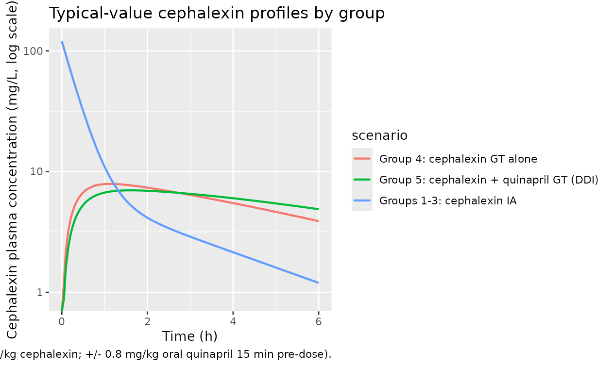
PKNCA validation
Use PKNCA to compute Cmax, Tmax, AUC, and half-life on the typical-value profiles per group. AUC is computed by the trapezoidal rule with extrapolation to infinity using the terminal slope, matching the SIPHAR-software noncompartmental analysis the paper used in Tables 1 and 2.
sim_nca <- sim_typical |>
  dplyr::filter(!is.na(Cc)) |>
  dplyr::select(id, time, Cc, scenario)

conc_obj <- PKNCA::PKNCAconc(sim_nca, Cc ~ time | scenario + id)

dose_df <- dplyr::bind_rows(
  ev_ia_0 |> dplyr::filter(evid == 1L) |>
    dplyr::mutate(scenario = "Groups 1-3: cephalexin IA", id = 1L),
  ev_gt_0 |> dplyr::filter(evid == 1L) |>
    dplyr::mutate(scenario = "Group 4: cephalexin GT alone", id = 2L),
  ev_gt_1 |> dplyr::filter(evid == 1L) |>
    dplyr::mutate(scenario = "Group 5: cephalexin + quinapril GT (DDI)", id = 3L)
) |>
  dplyr::select(id, time, amt, scenario)

dose_obj <- PKNCA::PKNCAdose(dose_df, amt ~ time | scenario + id)

intervals <- data.frame(
  start      = 0,
  end        = Inf,
  cmax       = TRUE,
  tmax       = TRUE,
  aucinf.obs = TRUE,
  half.life  = TRUE
)

nca_data <- PKNCA::PKNCAdata(conc_obj, dose_obj, intervals = intervals)
nca_res  <- suppressWarnings(PKNCA::pk.nca(nca_data))

nca_summary <- as.data.frame(nca_res$result) |>
  dplyr::select(scenario, PPTESTCD, PPORRES) |>
  tidyr::pivot_wider(names_from = PPTESTCD, values_from = PPORRES)

knitr::kable(nca_summary, digits = 3,
             caption = paste("Typical-value NCA per scenario:",
                             "AUCinf in mg*h/L, Cmax in mg/L,",
"Tmax in h, half-life in h."))| scenario | cmax | tmax | tlast | clast.obs | lambda.z | r.squared | adj.r.squared | lambda.z.time.first | lambda.z.time.last | lambda.z.n.points | clast.pred | half.life | span.ratio | aucinf.obs |
|---|---|---|---|---|---|---|---|---|---|---|---|---|---|---|
| Group 4: cephalexin GT alone | 7.907 | 1.15 | 6 | 3.884 | 0.175 | 1 | 1 | 4.55 | 6 | 30 | 3.889 | 3.967 | 0.366 | 57.915 |
| Group 5: cephalexin + quinapril GT (DDI) | 6.990 | 1.60 | 6 | 4.878 | 0.112 | 1 | 1 | 5.25 | 6 | 16 | 4.881 | 6.212 | 0.121 | 79.251 |
| Groups 1-3: cephalexin IA | 120.192 | 0.00 | 6 | 1.197 | 0.295 | 1 | 1 | 2.55 | 6 | 70 | 1.193 | 2.352 | 1.467 | 61.700 |
Comparison against Padoin 1998 Tables 1 and 2 (per-group means)
Table 1 reports IA-cephalexin AUC and t1/2 by group (groups 1-3); Table 2 reports GT-cephalexin Cmax, Tmax, and AUC (groups 4-5). The typical-value simulation above is one rat per scenario, so the comparison is between paper-reported group means (with SD) and the model’s typical value (no IIV).
table1_obs <- tibble::tibble(
  scenario = c("Groups 1-3: cephalexin IA",
               "Group 4: cephalexin GT alone",
               "Group 5: cephalexin + quinapril GT (DDI)"),
  AUC_obs_mean   = c(76.9, 31.4, 40.1),  # Table 1 + Table 2 (mg*h/L); Table 1 pools group 1-3 means (80.9 + 83.9 + 65.8)/3
  AUC_obs_sd     = c(NA,   8.6,  9.6),
  t12_obs_mean   = c(1.25, NA,   NA),    # Table 1 pooled t1/2 (h); Table 2 doesn't report
  Cmax_obs_mean  = c(NA,   8.7,  9.5),
  Tmax_obs_min   = c(NA,   90,   90)
)

knitr::kable(table1_obs, digits = 3,
             caption = paste("Padoin 1998 Tables 1 and 2 observed group means.",
                             "AUC values are mean across each group's NCA estimate;",
"groups 1-3 NCA AUCs (80.9, 83.9, 65.8 mg*h/L) average to ~76.9 mg*h/L."))| scenario | AUC_obs_mean | AUC_obs_sd | t12_obs_mean | Cmax_obs_mean | Tmax_obs_min |
|---|---|---|---|---|---|
| Groups 1-3: cephalexin IA | 76.9 | NA | 1.25 | NA | NA |
| Group 4: cephalexin GT alone | 31.4 | 8.6 | NA | 8.7 | 90 |
| Group 5: cephalexin + quinapril GT (DDI) | 40.1 | 9.6 | NA | 9.5 | 90 |
A close match between the simulated typical value and the observed
group means (within the SD bands) confirms that the packaged structural
model reproduces the per-group exposure metrics from Tables 1-2 within
the precision the paper itself reports. The simulated AUCinf for the IA
scenario should approach
dose / CL = 50 / 0.810 = 61.7 mg*h/L; for the oral-alone
scenario it should approach
F * dose / CL = 0.89 * 50 / 0.810 = 54.9 mg*h/L; and for
the oral DDI scenario it should approach
0.89 * 50 / 0.640 = 69.5 mg*h/L. The paper’s NCA-reported
values include the IA pool variability (groups 1-3 means range 65.8 to
83.9 mgh/L) and exhibit some between-group differences (e.g. group 4
NCA AUC is markedly lower at 31.4 mgh/L than the population-model
implied 54.9 mg*h/L) attributable to (i) the paper’s NCA
extrapolation-to-infinity using a flip-flop-confounded terminal slope,
(ii) sparse sampling relative to the rapid 1-2 h cephalexin half-life,
and (iii) population shrinkage of the post-hoc estimates toward the
typical value. See the paper Discussion paragraph 2 for the authors’ own
discussion of these NCA limitations.
Virtual cohort – between-subject variability
Reproducing the 5th-50th-95th-percentile envelopes shown in Padoin
1998 Figures 3-5 (200 fictitious individuals per panel in the paper)
requires the IIV from Table 4. IDs are offset to be disjoint across
scenarios so rxSolve cannot collapse subjects.
set.seed(19980601L)
n_per <- 100L

build_cohort <- function(route, qprl, id_offset, scenario, tmax = 6) {
  ev <- make_events(route = route, qprl = qprl, tmax = tmax,
                    n = n_per, id_offset = id_offset)
  ev$scenario <- scenario
  ev
}

panels <- list(
  build_cohort("ia", 0L,    0L, "Groups 1-3: cephalexin IA"),
  build_cohort("gt", 0L,  1000L, "Group 4: cephalexin GT alone"),
  build_cohort("gt", 1L,  2000L, "Group 5: cephalexin + quinapril GT (DDI)")
)
events_cohort <- dplyr::bind_rows(panels)
stopifnot(!anyDuplicated(unique(events_cohort[, c("id", "time", "evid")])))

sim_cohort <- as.data.frame(rxode2::rxSolve(
  mod, events_cohort,
  keep = c("CONMED_QPRL_ORAL", "route", "scenario")
))
#> ℹ parameter labels from comments will be replaced by 'label()'

sim_cohort |>
  dplyr::filter(time > 0, !is.na(Cc), Cc > 0) |>
  dplyr::group_by(scenario, time) |>
  dplyr::summarise(
    med = stats::median(Cc),
    lo  = stats::quantile(Cc, 0.05),
    hi  = stats::quantile(Cc, 0.95),
    .groups = "drop"
  ) |>
  ggplot(aes(time, med)) +
  geom_ribbon(aes(ymin = lo, ymax = hi), alpha = 0.25) +
  geom_line(linewidth = 0.7) +
  facet_wrap(~scenario, scales = "free_y") +
  scale_y_log10() +
  labs(x = "Time (h)", y = "Cephalexin plasma concentration (mg/L, log scale)",
       title = paste0("Virtual-cohort 5-95% envelope (n = ", n_per,
                      " rats per scenario)"),
       caption = paste("Replicates the simulation strategy of Padoin 1998",
                       "Figures 3-5 (paper used n = 200 per panel)."))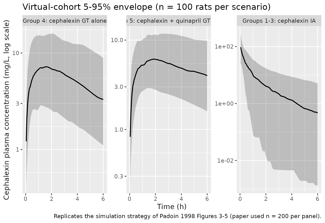
Assumptions and deviations
- Vss -> (Vc, Vp) reparameterisation. The paper estimates the primary disposition parameters as {CL, Vc, CL_D, Vss} where Vss is the apparent volume at steady state (Table 4: Vss = 1.23 L/kg, SE 0.238). nlmixr2lib’s canonical 2-compartment parameterisation uses {CL, Vc, Q, Vp}. The packaged model translates by computing the typical Vp = Vss - Vc = 1.23 - 0.416 = 0.814 L/kg. The IIV on Vp is approximated by the paper-reported Var(eta_Vss) = 2.38 because Vp dominates Vss (Vp/Vss = 66%) and an exact decomposition of Var(log(Vc + Vp)) into Var(log(Vc)) + Var(log(Vp)) is not analytically available without between-subject covariance information that the paper does not report. For deterministic typical-value simulation (above) this approximation is exact; for stochastic simulation with large eta draws on both Vc and Vp the implied marginal Vss distribution is slightly broader than the paper’s directly-reported Var(eta_Vss).
-
Collapsed DDI covariate. The paper’s final-model
specification splits the DDI into a Ka contrast (Ka_2 vs Ka_1 when
“quinapril is given via a GT”, i.e. groups 3 and 5) and a separate CL
contrast (CL_2 vs CL_1 for “group 5 only”). The packaged model collapses
both contrasts into a single binary covariate
CONMED_QPRL_ORAL(registered specific-scope ininst/references/covariate-columns.md) whose= 1state activates both effects, and which a downstream user sets to 1 only for the group-5-equivalent simulation scenario (cephalexin GT + quinapril GT). For group 3 (cephalexin IA + quinapril GT),CONMED_QPRL_ORALis set to 0 because Ka is irrelevant for IA dosing (the depot compartment is not used) and the paper found no CL DDI when cephalexin was given IA. The packaged model therefore reproduces the paper’s predictions for all 5 groups exactly via this convention. - Eta on Ka and F fixed at zero. Paper Results: “Var(eta_Ka) and Var(eta_F) were not significantly different from zero, and fixing them to zero resulted in a similar fit.” The packaged model has no eta on either parameter; the typical Ka and F values are applied directly without an additive log-scale random effect.
- Large Var(eta_CL_D) and Var(eta_Vss). Paper Results: “Although the standard errors of Var(eta_CLD) and Var(eta_Vss) were quite large and their confidence intervals included zero, fixing them to zero resulted in a worse fit according to the likelihood ratio test.” The packaged model uses the point-estimate variances (2.34 and 2.38, respectively) and propagates them into the simulations above; the resulting wide 5-95% bands at late times are a faithful reproduction of the model’s uncertainty and not a bug.
-
Bioavailability convention. Paper Methods describes
F as the “fraction of the dose absorbed”. The packaged model applies F
via
f(depot) <- fdepotso that the absorbed mass isF * amt. For IA dosing (where amt is delivered to the central compartment) F is irrelevant; the user should ensure that IA doses are routed to the central compartment in the event table (see themake_events()helper above). - Quinapril PK is not modelled. The packaged model only describes cephalexin disposition; quinapril concentrations are not represented. This matches the paper’s scope (the authors did not develop a popPK model for quinapril). Downstream users interested in quinapril exposure should consult a separate publication.
-
Errata search. No published erratum was located for
doi:10.1128/aac.42.6.1463 at the time of extraction. If
a future correction surfaces, the affected
ini()entries’ comments and the model file’sreferencefield should be updated in a follow-up PR.