Piperacillin (Bulitta 2007)
Source:vignettes/articles/Bulitta_2007_piperacillin.Rmd
Bulitta_2007_piperacillin.RmdModel and source
- Citation: Bulitta JB, Duffull SB, Kinzig-Schippers M, Holzgrabe U, Stephan U, Drusano GL, Sorgel F. Systematic comparison of the population pharmacokinetics and pharmacodynamics of piperacillin in cystic fibrosis patients and healthy volunteers. Antimicrob Agents Chemother. 2007;51(7):2497-2507. doi:10.1128/AAC.01477-06.
- Description: Two-compartment first-order IV population PK model for piperacillin in 8 adult cystic-fibrosis patients and 26 adult healthy volunteers receiving 4 g piperacillin as a 5-min intravenous infusion (Bulitta 2007). Lean body mass (LBM) is the size descriptor with allometric scaling (exponents 0.75 on CL and Q, 1.0 on V1 and V2; LBM_STD = 53 kg). A cystic-fibrosis disease-state indicator multiplicatively scales V1 and V2 via fcyf_vss^DIS_CF (fcyf_vss = 0.926), with fcyf_cl^DIS_CF retained on CL at its boundary estimate of 1.00 for model-form traceability.
- Article: https://doi.org/10.1128/AAC.01477-06
Population
The study enrolled 34 Caucasian adults at a single centre in Germany:
8 cystic-fibrosis (CF) patients (5 male, 3 female; age 21 +/- 4 years;
total body weight 43.1 +/- 7.8 kg; lean body mass [LBM] 37.2 +/- 6.9 kg;
body mass index 16.7 +/- 1.1 kg/m^2) and 26 healthy adult volunteers (13
male, 13 female; age 25 +/- 4 years; total body weight 71.1 +/- 11.8 kg;
LBM 56.4 +/- 7.2 kg; body mass index 23.6 +/- 3.7 kg/m^2). CF diagnosis
was confirmed by sweat test and clinical history; patients were studied
during an infection-free period and had no concomitant anti-infective
treatment. Each subject received a single 5-min IV infusion of 4 g
piperacillin (one CF patient received 3 g). Plasma piperacillin
concentrations were measured by HPLC at 21 nominal time points to 24 h
post-infusion (LOQ 0.200 mg/L). Demographics are from Bulitta 2007 Table
1. The same demographics are available programmatically via
readModelDb("Bulitta_2007_piperacillin")()$population.
The final structural model is a two-compartment first-order IV
disposition with lean body mass as the size descriptor (LBM_STD = 53 kg,
allometric exponents 0.75 on clearances and 1.0 on volumes; Bulitta 2007
Materials and Methods “Size models”). A cystic-fibrosis disease-state
indicator (DIS_CF) scales V1 and V2 multiplicatively by
fcyf_vss^DIS_CF with fcyf_vss = 0.926 (Table
4, LBM-allometric row); the corresponding clearance factor
fcyf_cl was estimated at the model boundary 1.00 and is
retained in the encoding for model-form traceability with no numerical
effect at the published point estimate.
Source trace
The per-parameter origin is recorded as an in-file comment next to
each ini() entry in
inst/modeldb/specificDrugs/Bulitta_2007_piperacillin.R. The
table below collects them in one place for review.
| Equation / parameter | Value | Source location |
|---|---|---|
lcl (typical CL, healthy, LBM = 53 kg) |
log(11.3) L/h |
Bulitta 2007 Table 3, “Estimates from original dataset” |
lvc (typical V1, healthy, LBM = 53 kg) |
log(7.01) L |
Bulitta 2007 Table 3 |
lvp (typical V2, healthy, LBM = 53 kg) |
log(3.37) L |
Bulitta 2007 Table 3 |
lq (typical CLic) |
log(12.8) L/h |
Bulitta 2007 Table 3 (CLic row) |
fcyf_cl (CF / healthy CL ratio) |
1.00 | Bulitta 2007 Table 4, LBM-allometric row (FCYF_CL; CI 0.92-1.09) |
fcyf_vss (CF / healthy V1, V2 ratio) |
0.926 | Bulitta 2007 Table 4, LBM-allometric row (FCYF_VSS; CI 0.82-1.02) |
e_lbm_cl / e_lbm_q (LBM allometric
exponent on clearances) |
0.75 (fixed) | Bulitta 2007 Methods, “Size models” |
e_lbm_vc / e_lbm_vp (LBM allometric
exponent on volumes) |
1.00 (fixed) | Bulitta 2007 Methods, “Size models” |
lbm_std (reference LBM) |
53 kg (fixed) | Bulitta 2007 Methods, “Size models” |
etalcl (BSV CL, log-normal) |
10.4% CV -> omega^2 = 0.010758 | Bulitta 2007 Table 3 |
etalvc + etalvp (BSV V1, V2 with correlation) |
26.0% / 34.2% CV, r = -0.80 | Bulitta 2007 Table 3 and footnote e |
propSd (proportional residual) |
0.132 | Bulitta 2007 Table 3 (CVC = 13.2%) |
addSd (additive residual) |
1.88 mg/L | Bulitta 2007 Table 3 (SDC = 1.88 mg/L) |
| ODE system: two-compartment IV with first-order elimination | n/a | Bulitta 2007 Results, “Population PK analysis” |
| Zero-order input duration (TK0) | 5 min (fixed; supplied via the event table) | Bulitta 2007 Table 3 (TK0) |
Virtual cohort
Original observed data are not publicly available. The figures below use virtual populations whose covariate distributions approximate the published demographics: 100 CF patients with LBM ~ Normal(37.2, 6.9) kg and 200 healthy participants with LBM ~ Normal(56.4, 7.2) kg, each dosed with a single 4 g piperacillin IV infusion over 5 min.
set.seed(20260607)

n_cf      <- 100L
n_healthy <- 200L

obs_grid <- c(
  0,
  5 / 60,                                # end of 5-min infusion
  (5 + c(5, 10, 15, 20, 30, 45, 60, 90)) / 60,  # min post-end -> hours
  5/60 + c(2, 2.5, 3, 3.5, 4, 5, 6, 8, 10, 12, 24)
)
obs_grid <- sort(unique(obs_grid))

make_cohort <- function(n, lbm_mean, lbm_sd, dis_cf, cohort_label,
                        dose_mg = 4000, infusion_min = 5, id_offset = 0L) {
  ids <- id_offset + seq_len(n)
  lbm_per <- pmax(15, rnorm(n, mean = lbm_mean, sd = lbm_sd))

  # Dose row: IV infusion into the central compartment. `dur` (hours) sets
  # the zero-order input duration; piperacillin enters cmt = "central"
  # since the model has no depot.
  dose_rows <- data.frame(
    id     = ids,
    time   = 0,
    evid   = 1L,
    amt    = dose_mg,
    dur    = infusion_min / 60,
    cmt    = "central",
    LBM    = lbm_per,
    DIS_CF = dis_cf,
    cohort = cohort_label
  )

  # Observation rows: one row per subject per nominal sampling time.
  obs_rows <- expand.grid(
    id   = ids,
    time = obs_grid,
    KEEP.OUT.ATTRS = FALSE,
    stringsAsFactors = FALSE
  )
  obs_rows$evid   <- 0L
  obs_rows$amt    <- NA_real_
  obs_rows$dur    <- NA_real_
  obs_rows$cmt    <- "Cc"
  obs_rows$LBM    <- lbm_per[match(obs_rows$id, ids)]
  obs_rows$DIS_CF <- dis_cf
  obs_rows$cohort <- cohort_label

  rbind(dose_rows, obs_rows)
}

events <- dplyr::bind_rows(
  make_cohort(n_cf,      lbm_mean = 37.2, lbm_sd = 6.9, dis_cf = 1L,
              cohort_label = "CF",      id_offset = 0L),
  make_cohort(n_healthy, lbm_mean = 56.4, lbm_sd = 7.2, dis_cf = 0L,
              cohort_label = "Healthy", id_offset = n_cf)
)
stopifnot(!anyDuplicated(unique(events[, c("id", "time", "evid")])))

events <- events[order(events$id, events$time, -events$evid), ]
Simulation
mod <- readModelDb("Bulitta_2007_piperacillin")()
sim <- rxode2::rxSolve(mod, events = events, keep = c("cohort", "LBM", "DIS_CF"))
sim <- as.data.frame(sim)
For deterministic typical-value replication (Figure 1 of the paper, which shows the average concentration-time profile), zero the random effects:
mod_typ <- rxode2::zeroRe(mod)
sim_typ <- rxode2::rxSolve(mod_typ, events = events, keep = c("cohort"))
#> ℹ omega/sigma items treated as zero: 'etalcl', 'etalvc', 'etalvp'
#> Warning: multi-subject simulation without without 'omega'
sim_typ <- as.data.frame(sim_typ)
Replicate published figures
Figure 1 -typical concentration-time profile by cohort
typ_summary <- sim_typ |>
  dplyr::filter(time > 0) |>
  dplyr::group_by(time, cohort) |>
  dplyr::summarise(Cc_typ = mean(Cc), .groups = "drop")

ggplot(typ_summary, aes(time, Cc_typ, colour = cohort)) +
  geom_line(linewidth = 0.7) +
  geom_point(size = 1.4) +
  scale_y_log10() +
  labs(x = "Time post end of infusion (h)",
       y = "Piperacillin Cc (mg/L), typical",
       title = "Figure 1 -typical concentration-time profile",
       colour = "Cohort",
       caption = "Replicates Figure 1 of Bulitta 2007 (average plasma piperacillin in CF patients and healthy volunteers after 4 g IV over 5 min). Random effects zeroed; LBM at cohort mean.")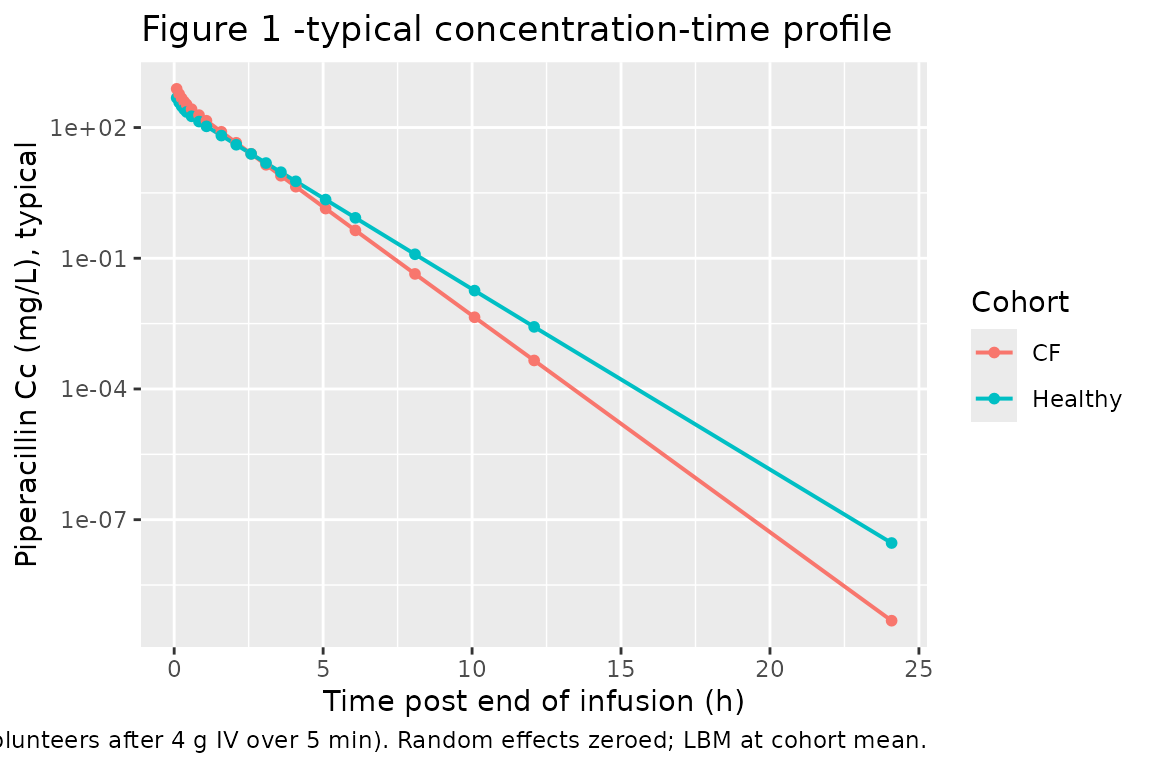
Figure 2 -visual predictive check (full-cohort VPC)
vpc <- sim |>
  dplyr::filter(time > 0) |>
  dplyr::group_by(time, cohort) |>
  dplyr::summarise(
    Q10 = quantile(Cc, 0.10, na.rm = TRUE),
    Q25 = quantile(Cc, 0.25, na.rm = TRUE),
    Q50 = quantile(Cc, 0.50, na.rm = TRUE),
    Q75 = quantile(Cc, 0.75, na.rm = TRUE),
    Q90 = quantile(Cc, 0.90, na.rm = TRUE),
    .groups = "drop"
  )

ggplot(vpc, aes(time, Q50)) +
  geom_ribbon(aes(ymin = Q10, ymax = Q90), alpha = 0.15) +
  geom_ribbon(aes(ymin = Q25, ymax = Q75), alpha = 0.30) +
  geom_line() +
  facet_wrap(~cohort) +
  scale_y_log10() +
  labs(x = "Time post end of infusion (h)",
       y = "Piperacillin Cc (mg/L)",
       title = "Figure 2 -VPC by cohort (10%, 25%, 50%, 75%, 90% percentiles)",
       caption = "Replicates Figure 2 of Bulitta 2007 (visual predictive check of the two-compartment LBM-allometric model).")
#> Warning in transformation$transform(x): NaNs produced
#> Warning in scale_y_log10(): log-10 transformation introduced infinite values.
#> Warning: Removed 1 row containing missing values or values outside the scale range
#> (`geom_ribbon()`).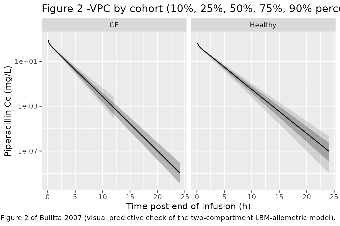
PKNCA validation
NCA on the simulated single-dose profiles. The paper’s Table 2 reports total clearance, V_SS, peak concentration, terminal half-life, and mean residence time as medians (range) per cohort; the simulated counterparts should fall close to those medians since the model was fit to the same data.
sim_nca <- sim |>
  dplyr::filter(!is.na(Cc), time > 0) |>
  dplyr::select(id, time, Cc, cohort)

dose_df <- events |>
  dplyr::filter(evid == 1L) |>
  dplyr::select(id, time, amt, cohort)

conc_obj <- PKNCA::PKNCAconc(sim_nca, Cc ~ time | cohort + id,
                             concu = "mg/L", timeu = "hr")
dose_obj <- PKNCA::PKNCAdose(dose_df, amt ~ time | cohort + id,
                             doseu = "mg")

intervals <- data.frame(
  start       = 0,
  end         = Inf,
  cmax        = TRUE,
  tmax        = TRUE,
  aucinf.obs  = TRUE,
  half.life   = TRUE,
  cl.obs      = TRUE,
  vss.obs     = TRUE,
  mrt.last    = TRUE
)

nca_res <- PKNCA::pk.nca(
  PKNCA::PKNCAdata(conc_obj, dose_obj, intervals = intervals)
)

nca_long <- as.data.frame(nca_res$result) |>
  dplyr::filter(PPTESTCD %in% c("cmax", "tmax", "aucinf.obs",
                                "half.life", "cl.obs", "vss.obs",
                                "mrt.last"))

nca_summary <- nca_long |>
  dplyr::group_by(cohort, PPTESTCD) |>
  dplyr::summarise(median = median(PPORRES, na.rm = TRUE),
                   q_lo   = quantile(PPORRES, 0.10, na.rm = TRUE),
                   q_hi   = quantile(PPORRES, 0.90, na.rm = TRUE),
                   .groups = "drop")

knitr::kable(nca_summary,
             digits = 3,
caption = "Simulated NCA parameters (median and 10-90% range) per cohort.")| cohort | PPTESTCD | median | q_lo | q_hi |
|---|---|---|---|---|
| CF | aucinf.obs | NA | NA | NA |
| CF | cl.obs | NA | NA | NA |
| CF | cmax | 773.649 | 549.762 | 1020.724 |
| CF | half.life | 0.633 | 0.529 | 0.756 |
| CF | mrt.last | NA | NA | NA |
| CF | tmax | 0.083 | 0.083 | 0.083 |
| CF | vss.obs | NA | NA | NA |
| Healthy | aucinf.obs | NA | NA | NA |
| Healthy | cl.obs | NA | NA | NA |
| Healthy | cmax | 456.374 | 333.109 | 642.968 |
| Healthy | half.life | 0.763 | 0.635 | 0.898 |
| Healthy | mrt.last | NA | NA | NA |
| Healthy | tmax | 0.083 | 0.083 | 0.083 |
| Healthy | vss.obs | NA | NA | NA |
Comparison against Bulitta 2007 Table 2
Published noncompartmental medians (range) from Bulitta 2007 Table 2:
| Parameter | CF patients (median, range) | Healthy (median, range) |
|---|---|---|
| Total clearance (L/h) | 8.78 (6.39-12.1) | 11.7 (6.25-14.5) |
| Volume of distribution at steady state (L) | 8.13 (5.16-10.8) | 11.8 (9.06-30.6) |
| Peak concentration (mg/L) | 767 (408-1044) | 446 (272-721) |
| Terminal half-life (h) | 0.69 (0.34-1.19) | 1.05 (0.49-7.52) |
| Mean residence time (h) | 0.85 (0.66-1.03) | 1.02 (0.79-3.49) |
The simulated values above were generated from a virtual cohort with the published demographic means and the published parameter point estimates; they should fall close to the published medians. Differences of more than ~20% from the published median in either cohort would warrant investigation; small deviations are expected because the virtual cohort uses a normal LBM distribution while the source cohort was a small finite sample (n = 8 CF, n = 26 healthy).
Assumptions and deviations
- LBM distribution modelled as Normal(mean, SD) per cohort, truncated below 15 kg. The source paper reports mean +/- SD for LBM (Table 1) but not the distribution shape; Normal is the most common assumption for body-size demographics at the adult-cohort scale.
- Sex, age, height, and BSA covariates are not modelled. The final Bulitta 2007 model retained only LBM and DIS_CF as covariates; other baseline characteristics were screened and did not enter the final model.
- Single 4 g infusion for all simulated subjects. One CF patient in the original study received 3 g; the cohort-level NCA summary is insensitive to this individual deviation because total clearance and V_SS are dose-normalised quantities.
-
fcyf_clretained at 1.00. The published estimate for the LBM- allometric final model was 1.00 (90% CI 0.92-1.09); it is included in the model file for model-form traceability and to preserve the published equation form, but the multiplier1.00^DIS_CFis 1 by construction so the encoded effect on CL is numerically zero at the point estimate. -
Zero-order infusion duration (TK0 = 5 min) is
supplied via the
durfield in the event table, not as a structural model parameter. Bulitta 2007 Table 3 lists TK0 = 5 min as fixed for the study’s actual infusion regimen; downstream users running a different infusion duration (e.g. 30 min short-term infusion or 4 h prolonged infusion as in the paper’s Monte Carlo PD section) should setduraccordingly. -
Monte Carlo PD breakpoints not reproduced. The
paper’s Monte Carlo simulations of probability-of-target-attainment
versus MIC and the derived PKPD breakpoints (Tables 6 and 7) require a
steady-state PD workflow that is outside the scope of this validation
vignette. The packaged model supplies the PK part of that workflow;
users wanting to replicate the PD breakpoints can simulate steady-state
dosing trajectories from the same
readModelDb("Bulitta_2007_piperacillin")object, apply the protein-binding fraction (30%, fixed in the paper), and integrate fT > MIC themselves.