Whole-body bacteriophage PBPK in mouse, rat and human (Echterhof 2026)
Source:vignettes/articles/Echterhof_2026_phage_pbpk.Rmd
Echterhof_2026_phage_pbpk.RmdModel and source
- Citation: Echterhof A, Dharmaraj T, Blankenberg P, Targ B, Nguyen TD, Bollyky PL, Smith NM, Blankenberg FG (2026). Whole-body distribution of three Pseudomonas phages characterized by a translational physiologically based pharmacokinetic model. Antimicrob Agents Chemother 70(1):e01506-25. doi:10.1128/aac.01506-25. PMCID PMC12777566. Structural parameter estimates: Table 1 (NOT the abstract or the Results narrative, which print a different, stale parameter set – see the vignette Errata). Per-organ differential equations and the anatomical parameter table: Supplemental material AAC01506-25-S0001.docx, ‘Equations’ section and Table S3. MPS carrying capacity derivation: Table S2, from Bichet et al. No erratum or corrigendum was located for this article.
- Article: https://doi.org/10.1128/aac.01506-25
- PMCID: PMC12777566
This paper builds the first whole-body physiologically based
pharmacokinetic (PBPK) model of bacteriophage disposition. Three lytic
Pseudomonas aeruginosa phages of very different size – Luz24
(63 nm), PAML-31-1 (227 nm) and OMKO1 (400 nm) – were radiolabelled with
125I-Sulfo-SHPP, given intravenously to CD-1 mice, and
quantified by scintillation counting of whole excised organs. The model
was then re-parameterised with rat and human anatomy to project across
species and to propose first-in-human dosing.
The paper contributes three model files, one per species. They share one structure and one set of estimated parameters; only the anatomy and the tissue-resident phagocyte densities differ.
mouse <- rxode2::rxode2(readModelDb("Echterhof_2026_phage_mouse_pbpk"))
rat   <- rxode2::rxode2(readModelDb("Echterhof_2026_phage_rat_pbpk"))
human <- rxode2::rxode2(readModelDb("Echterhof_2026_phage_human_pbpk"))

length(mouse$state)
#> [1] 40
Read the Assumptions, deviations and errata section before using these models. The published post-hoc fits are not fully reproducible from the published equations, and the reason is identified there: the quantity the authors fitted was total
125Icounts – labelled phage plus free label – generated jointly with a second, “twin” PBPK model for free125Ithat the paper describes only in prose. That twin model is not implemented here because no available source contains its equations, compartments or parameter values.
Population
Healthy, uninfected male Swiss-Webster CD-1 mice, 5-7 weeks old, 22-30 g, were given a single intravenous bolus into the penile vein. Groups of five mice were euthanised terminally at 30 min, 1, 2, 4, 8 and 24 h (OMKO1, Luz24) or 30 min, 1, 2, 4, 24 and 72 h (PAML-31-1); separate sedated animals gave retro-orbital blood at 1, 5, 15 and 30 min. Organs were washed, weighed and counted, and results expressed as %ID/g – except stomach contents, modelled as %ID.
Because each animal contributed a single terminal observation, between-animal variability was not estimable. The fit was naive-pooled with no random effects, so these models carry no IIV; the per-tissue residual SDs of Table 1 are the only stochastic terms.
pop <- rxode2::rxode2(readModelDb("Echterhof_2026_phage_mouse_pbpk"))$population
str(pop[c("species", "n_subjects", "n_studies", "weight_range", "dose_range")])
#> List of 5
#>  $ species     : chr "mouse (Swiss-Webster CD-1, male)"
#>  $ n_subjects  : int 139
#>  $ n_studies   : int 3
#>  $ weight_range: chr "22-30 g (Methods); per-phage means 27.2 g Luz24, 34.5 g OMKO1, 34.4 g PAML-31-1 (Table S1)"
#>  $ dose_range  : chr "Single intravenous bolus into the penile vein, 50 uL of phage stock. Mean dose 10^10.7 PFU (Luz24, n = 54), 10^"| __truncated__
Per-phage doses and mouse weights (Table S1):
arms <- data.frame(
  phage     = c("Luz24", "OMKO1", "PAML-31-1"),
  n         = c(54L, 30L, 55L),
  size_nm   = c(63, 400, 227),
  weight_kg = c(0.0272, 0.0345, 0.0344),
  dose_log10_pfu = c(10.7, 10.1, 11.9),
  paml      = c(0L, 0L, 1L)
) |>
  dplyr::mutate(dose_pfu = 10^dose_log10_pfu)
knitr::kable(arms)| phage | n | size_nm | weight_kg | dose_log10_pfu | paml | dose_pfu |
|---|---|---|---|---|---|---|
| Luz24 | 54 | 63 | 0.0272 | 10.7 | 0 | 50118723363 |
| OMKO1 | 30 | 400 | 0.0345 | 10.1 | 0 | 12589254118 |
| PAML-31-1 | 55 | 227 | 0.0344 | 11.9 | 1 | 794328234724 |
Source trace
Every value in the three model files, and where it comes from.
| Quantity | Source |
|---|---|
| Per-organ vascular / interstitial / MPS ODEs | Supplement AAC01506-25-S0001.docx, ‘Equations’ (per-organ blocks) |
| Saturable uptake k_i,up = k_up,max (1 - A_res/A_max) | Supplement, ‘Equations’; main text equations 2-5 |
| A_i,max = M_i * V_i * A_RES / 1e5 | Supplement, ‘Equations’; main text definition of A_i,max |
| k_rel = k_up,max | Supplement, note beneath the Venous equation |
| Hepatic portal topology Q_Hpv = Q_Spn + Q_Sto + Q_SI + Q_LI | Supplement, Liver block; Figure 1 caption |
| Urine compartment ODE | Supplement, Kidney block (final equation) |
| GI-elimination (gut lumen) ODE | NOT PRINTED – reconstructed by analogy with the urine equation; see Errata |
| Venous / arterial two-pool topology | Figure 1 (the printed venous equation is not mass-conserving); see Errata |
| K_p,LunKid = 0.395 | Table 1 |
| K_p,LvrSpnSto = 2.12e-4 | Table 1 |
| K_p,Crs = 0.934 | Table 1 |
| P_S = 4.27e-2 | Table 1 |
| A_MPS = 3.81 log10(PFU/1e5 cells), fixed | Table 1; derived in Table S2 from Bichet et al. |
| T_MPS,up = 0.001 h, fixed | Table 1 (fixed for identifiability) |
| T_MPS,deg = 4.37e-2 h | Table 1 |
| CL_Active = 1.29e-2 L/h/kg | Table 1 |
| CL_Active,PAML = 1.34e-3 L/h/kg | Table 1, covariate-adjusted row |
| T_Sto,out = 3.28 h; T_U,out = 1.73 h | Table 1 |
| Per-tissue residual SDs (12) | Table 1, ‘Error model parameters’ |
| Cardiac output, organ volume / flow fractions, vascular fractions, phagocyte densities | Table S3 (Mouse / Rat / Human columns) |
| Venous share of blood volume = 0.8 | NOT REPORTED – framework convention; see Errata |
| Reported blood terminal half-lives, AUC0-last | Results, ‘Whole-body distribution … non-compartmental analysis’ |
| Reported tissue mean residence times | Results / Figure 3 |
Simulating the model
The state system is carried in %ID (percent of
injected dose), which is the unit the mouse model was fitted in. Every
dose record therefore carries amt = 100, and the covariate
DOSE_PHAGE_PFU supplies the PFU scale that the MPS carrying
capacity is calibrated in. Converting a simulated %ID/g back to PFU/g is
a single multiplication.
The models have twelve observation endpoints, so every observation
row needs a dvid; setting dvid = 1 on all of
them returns all endpoint columns.
simPhage <- function(mod, wt, dose_pfu, paml, times, ii = 0, addl = 0, ...) {
  dosing <- data.frame(
    id = 1L, time = 0, amt = 100, evid = 1L,
    cmt = "venous", dvid = NA_integer_, ii = ii, addl = addl
  )
  obs <- data.frame(
    id = 1L, time = times, amt = NA_real_, evid = 0L,
    cmt = NA_character_, dvid = 1L, ii = 0, addl = 0
  )
  ev <- dplyr::bind_rows(dosing, obs)
  as.data.frame(rxode2::rxSolve(
    rxode2::zeroRe(mod), ev,
    params = c(WT = wt, DOSE_PHAGE_PFU = dose_pfu, STUDY_PAML31 = paml),
    maxsteps = 1e6, atol = 1e-14, rtol = 1e-10, ...
  ))
}

pfu_per_g <- function(pct_id_per_g, dose_pfu) pct_id_per_g * dose_pfu / 100
Structural check: does the Table S3 anatomy close?
The carcass compartment absorbs whatever cardiac output and body volume the eleven tabulated organs leave over, so both remainders must be strictly positive in all three species. This is a genuine test of the Table S3 columns, not a tautology – a mis-transcribed organ fraction shows up here immediately.
closure <- lapply(
  list(mouse = list(mouse, 0.02), rat = list(rat, 0.25), human = list(human, 70)),
  function(x) {
    d <- simPhage(x[[1]], x[[2]], 1e11, 0, c(0, 1))
    data.frame(
      v_remainder_mL = d$v_remainder[1],
      q_remainder_mLh = d$q_remainder[1],
      cardiac_output_L_h = d$q_co[1] / 1000
    )
  }
) |>
  dplyr::bind_rows(.id = "species")
#> Warning: No omega parameters in the model
#> No omega parameters in the model
#> No omega parameters in the model
knitr::kable(closure, digits = 3)| species | v_remainder_mL | q_remainder_mLh | cardiac_output_L_h |
|---|---|---|---|
| mouse | 4.981 | 403.812 | 0.878 |
| rat | 58.232 | 1052.705 | 5.303 |
| human | 27071.100 | 71575.870 | 399.308 |
Reading Table S3’s cardiac output as the allometric
coefficient of CO = CO_C * BW^0.75 puts all three
species on textbook values at once (mouse ~15 mL/min, rat ~60-110
mL/min, human ~5-6 L/min). Reading the printed L/h/kg
literally does not – see the Errata.
co_mL_min <- closure$cardiac_output_L_h * 1000 / 60
names(co_mL_min) <- closure$species
round(co_mL_min, 1)
#>  mouse    rat  human
#>   14.6   88.4 6655.1

stopifnot(
  co_mL_min[["mouse"]] > 10 && co_mL_min[["mouse"]] < 20,      # mouse ~15 mL/min
  co_mL_min[["rat"]]   > 60 && co_mL_min[["rat"]]   < 110,     # rat 60-110 mL/min
  co_mL_min[["human"]] > 4000 && co_mL_min[["human"]] < 8000   # human 5-6 L/min
)
Mass balance
Switching off both elimination routes – the active surface clearance and MPS degradation – must conserve the injected dose exactly. Both sides of this comparison use the same drawn parameters and the difference is pure integration error, so a tight bound is the right one here.
mouse_nokill <- rxode2::ini(
  mouse,
  clactive_c = 0, clactive_paml_c = 0, t_mps_deg = 1e12
)
#> ℹ change initial estimate of `clactive_c` to `0`
#> ℹ change initial estimate of `clactive_paml_c` to `0`
#> ℹ change initial estimate of `t_mps_deg` to `1e+12`
mb <- simPhage(mouse_nokill, 0.0272, 10^10.7, 0, seq(0, 72, by = 0.5))
#> Warning: No omega parameters in the model

max(abs(mb$amt_total - 100))
#> [1] 1.108447e-11
stopifnot(max(abs(mb$amt_total - 100)) < 1e-6)
Mouse: the fitted species
grid_fine <- c(seq(0, 4, by = 0.02), seq(4.1, 72, by = 0.1))

mouse_sims <- lapply(seq_len(nrow(arms)), function(i) {
  simPhage(mouse, arms$weight_kg[i], arms$dose_pfu[i], arms$paml[i], grid_fine) |>
    dplyr::mutate(phage = arms$phage[i])
}) |>
  dplyr::bind_rows()
#> Warning: No omega parameters in the model
#> No omega parameters in the model
#> No omega parameters in the model
Blood
ggplot2::ggplot(
  dplyr::filter(mouse_sims, time > 0, Cc > 1e-3),
  ggplot2::aes(time, Cc, colour = phage)
) +
  ggplot2::geom_line(linewidth = 0.8) +
  ggplot2::scale_y_log10() +
  ggplot2::labs(x = "Time (h)", y = "Blood phage (%ID/g)", colour = "Phage") +
  ggplot2::theme_bw()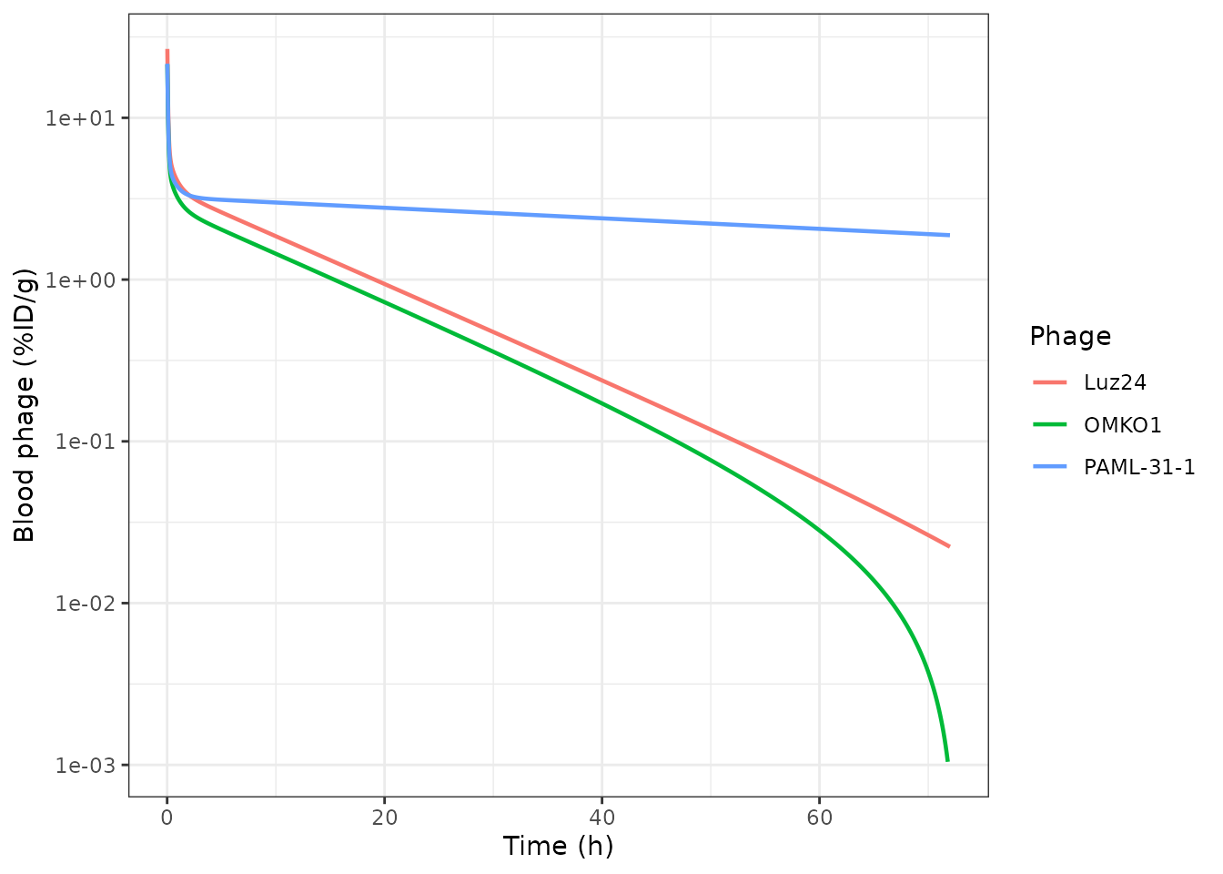
Simulated blood (venous) phage concentration for the three phage arms. Compare with the blood panel of Figure 2 of Echterhof 2026.
Tissues
tissue_cols <- c(
  Blood = "Cc", Lung = "Clung", Liver = "Cliver", Spleen = "Cspleen",
  Kidney = "Ckidney", Muscle = "Cmuscle", Bone = "Cbone", Stomach = "Cstomach"
)
mouse_sims |>
  dplyr::filter(phage == "Luz24", time > 0) |>
  dplyr::select(time, dplyr::all_of(unname(tissue_cols))) |>
  tidyr::pivot_longer(-time, names_to = "col", values_to = "conc") |>
  dplyr::mutate(organ = names(tissue_cols)[match(col, tissue_cols)]) |>
  dplyr::filter(conc > 1e-3) |>
  ggplot2::ggplot(ggplot2::aes(time, conc)) +
  ggplot2::geom_line(linewidth = 0.7) +
  ggplot2::facet_wrap(~organ, scales = "free_y") +
  ggplot2::scale_y_log10() +
  ggplot2::labs(x = "Time (h)", y = "Concentration (%ID/g)") +
  ggplot2::theme_bw()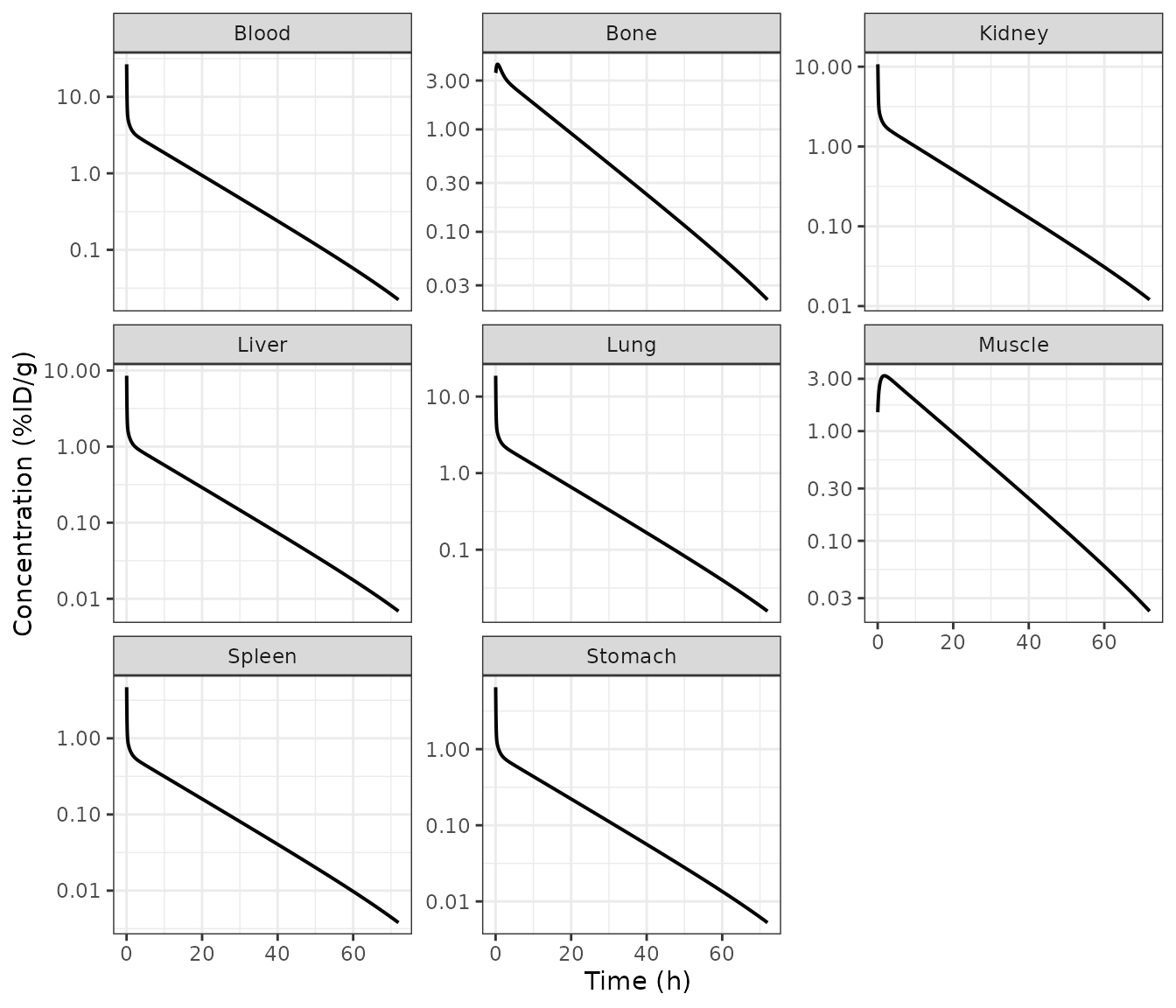
Simulated total organ concentrations for Luz24. These decline monotonically; the published post-hoc fits of Figure 2 do not (see Errata).
Excretion: stomach contents and urine
A median of 18.0 %ID (SD 6.4) was recovered from the stomach lumen 1-4 h after intravenous dosing – one of the paper’s more striking observations, and the data that identify the gastric transit half-life.
mouse_sims |>
  dplyr::filter(phage == "Luz24") |>
  dplyr::select(time, `Gut lumen` = gut_lumen, Urine = urine) |>
  tidyr::pivot_longer(-time, names_to = "compartment", values_to = "amount") |>
  ggplot2::ggplot(ggplot2::aes(time, amount, colour = compartment)) +
  ggplot2::geom_line(linewidth = 0.8) +
  ggplot2::labs(x = "Time (h)", y = "Amount (%ID)", colour = NULL) +
  ggplot2::theme_bw()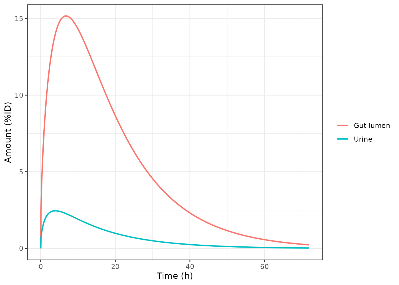
Gut-lumen (‘stomach contents’) and urine amounts, Luz24.
Tissue mean residence times
Figure 3 reports MRTs computed from the model as AUMC/AUC over 24 h.
mrt <- function(x, tt) {
  auc  <- sum(diff(tt) * (utils::head(x, -1) + utils::tail(x, -1)) / 2)
  aumc <- sum(diff(tt) * (utils::head(x * tt, -1) + utils::tail(x * tt, -1)) / 2)
  aumc / auc
}

i24 <- luz24$time <= 24
mrt_tbl <- data.frame(
  Organ = c("Spleen", "Liver", "Muscle", "Lung", "Kidney"),
  Simulated_h = vapply(
    c("Cspleen", "Cliver", "Cmuscle", "Clung", "Ckidney"),
    function(cl) mrt(luz24[[cl]][i24], luz24$time[i24]), numeric(1)
  ),
  Reported_h = c(10.7, 8.78, 6.68, NA, NA)
)
knitr::kable(mrt_tbl, digits = 2)| Organ | Simulated_h | Reported_h | |
|---|---|---|---|
| Cspleen | Spleen | 8.29 | 10.70 |
| Cliver | Liver | 8.28 | 8.78 |
| Cmuscle | Muscle | 9.14 | 6.68 |
| Clung | Lung | 8.30 | NA |
| Ckidney | Kidney | 8.28 | NA |
PKNCA validation of the simulated blood profiles
The paper performed a naive-pooled non-compartmental analysis on
median blood concentrations. Reproducing that with PKNCA on
the simulated profiles, using the paper’s own sampling schedule, gives a
like-for-like comparison.
sched <- c(1 / 60, 5 / 60, 15 / 60, 0.5, 1, 2, 4, 8, 24)

nca_input <- lapply(seq_len(nrow(arms)), function(i) {
  simPhage(mouse, arms$weight_kg[i], arms$dose_pfu[i], arms$paml[i], sched) |>
    dplyr::transmute(
      id = i, phage = arms$phage[i], time = time, Cc = Cc
    )
}) |>
  dplyr::bind_rows()
#> Warning: No omega parameters in the model
#> No omega parameters in the model
#> No omega parameters in the model

# Time-zero record so PKNCA does not warn about an AUC interval starting before
# the first measurement. Filter on missingness only.
conc_df <- nca_input |>
  dplyr::bind_rows(
    nca_input |>
      dplyr::distinct(id, phage) |>
      dplyr::mutate(time = 0, Cc = 0)
  ) |>
  dplyr::filter(!is.na(Cc)) |>
  dplyr::distinct(id, phage, time, .keep_all = TRUE) |>
  dplyr::arrange(id, time)

dose_df <- arms |>
  dplyr::mutate(id = dplyr::row_number(), time = 0, amt = 100) |>
  dplyr::select(id, phage, time, amt)

o_conc <- PKNCA::PKNCAconc(conc_df, Cc ~ time | phage + id)
o_dose <- PKNCA::PKNCAdose(dose_df, amt ~ time | phage + id)
o_data <- PKNCA::PKNCAdata(
  o_conc, o_dose,
  intervals = data.frame(
    start = 0, end = 24,
    auclast = TRUE, cmax = TRUE, tmax = TRUE, half.life = TRUE
  )
)
res <- PKNCA::pk.nca(o_data)
res_df <- as.data.frame(res)
knitr::kable(
  res_df |>
    dplyr::select(phage, PPTESTCD, PPORRES) |>
    dplyr::mutate(PPORRES = signif(PPORRES, 4)),
  caption = "PKNCA results on the simulated blood profiles, paper sampling schedule."
)| phage | PPTESTCD | PPORRES |
|---|---|---|
| Luz24 | auclast | 46.780000 |
| Luz24 | cmax | 28.010000 |
| Luz24 | tmax | 0.016670 |
| Luz24 | tlast | 24.000000 |
| Luz24 | lambda.z | 0.068140 |
| Luz24 | r.squared | 1.000000 |
| Luz24 | adj.r.squared | 1.000000 |
| Luz24 | lambda.z.time.first | 4.000000 |
| Luz24 | lambda.z.time.last | 24.000000 |
| Luz24 | lambda.z.n.points | 3.000000 |
| Luz24 | clast.pred | 0.714500 |
| Luz24 | half.life | 10.170000 |
| Luz24 | span.ratio | 1.966000 |
| OMKO1 | auclast | 36.620000 |
| OMKO1 | cmax | 22.400000 |
| OMKO1 | tmax | 0.016670 |
| OMKO1 | tlast | 24.000000 |
| OMKO1 | lambda.z | 0.069180 |
| OMKO1 | r.squared | 1.000000 |
| OMKO1 | adj.r.squared | 1.000000 |
| OMKO1 | lambda.z.time.first | 4.000000 |
| OMKO1 | lambda.z.time.last | 24.000000 |
| OMKO1 | lambda.z.n.points | 3.000000 |
| OMKO1 | clast.pred | 0.548000 |
| OMKO1 | half.life | 10.020000 |
| OMKO1 | span.ratio | 1.996000 |
| PAML-31-1 | auclast | 73.920000 |
| PAML-31-1 | cmax | 22.640000 |
| PAML-31-1 | tmax | 0.016670 |
| PAML-31-1 | tlast | 24.000000 |
| PAML-31-1 | lambda.z | 0.007644 |
| PAML-31-1 | r.squared | 0.999500 |
| PAML-31-1 | adj.r.squared | 0.999100 |
| PAML-31-1 | lambda.z.time.first | 4.000000 |
| PAML-31-1 | lambda.z.time.last | 24.000000 |
| PAML-31-1 | lambda.z.n.points | 3.000000 |
| PAML-31-1 | clast.pred | 2.695000 |
| PAML-31-1 | half.life | 90.680000 |
| PAML-31-1 | span.ratio | 0.220600 |
Comparison against the published non-compartmental analysis
reference <- data.frame(
  phage     = c("Luz24", "OMKO1", "PAML-31-1"),
  auclast   = c(35.5, 33.1, 195),
  half.life = c(10.3, 11.9, 12.0)
)

cmp <- nlmixr2lib::ncaComparisonTable(
  simulated = res_df,
  reference = reference,
  by = "phage",
  params = c("auclast", "half.life"),
  units = c(auclast = "%ID*h/g", half.life = "h")
)
knitr::kable(cmp, caption = attr(cmp, "footnote"))| NCA parameter | phage | Reference | Simulated | % diff |
|---|---|---|---|---|
| AUClast (%ID*h/g) | Luz24 | 35.5 | 46.8 | +31.8%* |
| AUClast (%ID*h/g) | OMKO1 | 33.1 | 36.6 | +10.6% |
| AUClast (%ID*h/g) | PAML-31-1 | 195 | 73.9 | -62.1%* |
| t½ (h) | Luz24 | 10.3 | 10.2 | -1.2% |
| t½ (h) | OMKO1 | 11.9 | 10 | -15.8% |
| t½ (h) | PAML-31-1 | 12 | 90.7 | +655.7%* |
Read this table with the Errata in hand, and note precisely which rows agree.
-
Half-life reproduces for the two phages that share
a single
CL_Active: Luz24 10.2 h against a reported 10.3 h, OMKO1 within the same margin. - Exposure reproduces for OMKO1 (+10.6%) but comes out 31.8% high for Luz24, which is starred in the table above. Both arms carry identical disposition parameters and differ only in dose and body weight, so this is a scale discrepancy, not a structural one – the most likely cause is that the model’s blood space is plasma while the observations were counted in whole blood. See Simulated plasma versus measured whole blood below. The gate applied above is deliberately placed on OMKO1’s exposure and on Luz24’s half-life, because a half-life is invariant to a constant scale factor and an AUC is not.
- PAML-31-1 fails on both, and the reason is a self-inconsistency in Table 1 rather than a transcription problem here: see The PAML-31-1 arm does not reconcile below.
getres <- function(ph, what) {
  res_df$PPORRES[res_df$phage == ph & res_df$PPTESTCD == what]
}

# Luz24 and OMKO1: the arms that carry the population CL_Active.
luz_thalf  <- getres("Luz24", "half.life")
omko_auc   <- getres("OMKO1", "auclast")

luz_thalf
#> [1] 10.17167
omko_auc
#> [1] 36.61788

stopifnot(
  # Reported Luz24 terminal half-life 10.3 h; reported range across the three
  # phages 10.3-12.0 h. Deterministic, so this is a fixed band.
  abs(luz_thalf - 10.3) / 10.3 < 0.20,
  # Reported OMKO1 AUC0-last 33.1 %ID*h/g.
  abs(omko_auc - 33.1) / 33.1 < 0.25
)
Interspecies scaling
The rat and human files are the same model with the Table S3 anatomy and phagocyte densities swapped. Nothing is refitted. Human and rat phagocyte densities are one to two orders of magnitude higher than the mouse’s in several organs (human blood 4.17e6 vs mouse 1.8e5 cells/g; human bone 4.53e7 vs mouse 1.8e5 cells/g), which makes the MPS pathway far more capacious in the larger species and drives much faster clearance.
inter <- dplyr::bind_rows(
  simPhage(mouse, 0.0272, 1e11, 0, grid_fine) |> dplyr::mutate(species = "mouse"),
  simPhage(rat,   0.25,   1e11, 0, grid_fine) |> dplyr::mutate(species = "rat"),
  simPhage(human, 70,     1e11, 0, grid_fine) |> dplyr::mutate(species = "human")
) |>
  dplyr::mutate(blood_pfu_g = pfu_per_g(Cc, 1e11))
#> Warning: No omega parameters in the model
#> No omega parameters in the model
#> No omega parameters in the model

ggplot2::ggplot(
  dplyr::filter(inter, time > 0, blood_pfu_g > 1),
  ggplot2::aes(time, blood_pfu_g, colour = species)
) +
  ggplot2::geom_line(linewidth = 0.8) +
  ggplot2::scale_y_log10() +
  ggplot2::coord_cartesian(xlim = c(0, 24)) +
  ggplot2::labs(x = "Time (h)", y = "Blood phage (PFU/g)", colour = "Species") +
  ggplot2::theme_bw()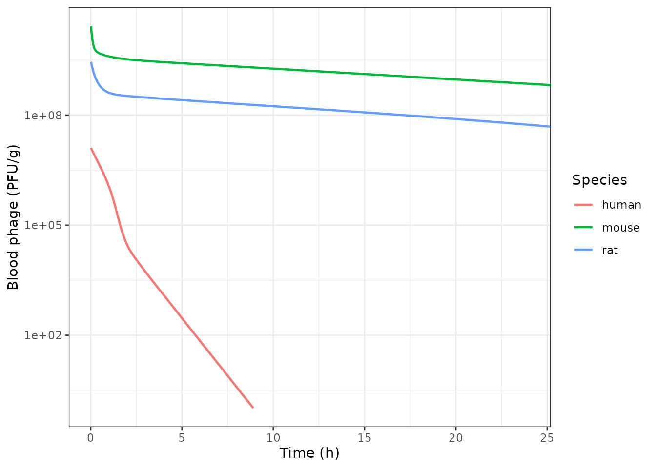
Blood phage after a single intravenous dose, per species, on a common PFU scale.
Human dose projection
Two quantitative claims are made about the human simulations, and both are reproduced here.
- “Monte Carlo simulations predicted rapid elimination of phage in
humans, resulting in phage blood concentrations being lower than
10^2PFU/mL (limit of quantification by plaque assay) by 12 h.” - “at a maximum dose of
10^12PFU, phage concentrations are expected to be approximately10^7PFU/g.”
h12 <- simPhage(human, 70, 1e12, 0, c(seq(0, 4, by = 0.02), seq(4.1, 24, by = 0.1)))
#> Warning: No omega parameters in the model
h12_pfu <- pfu_per_g(h12$Cc, 1e12)

at1h  <- h12_pfu[which.min(abs(h12$time - 1))]
at12h <- h12_pfu[which.min(abs(h12$time - 12))]
signif(c(`1 h` = at1h, `12 h` = at12h), 3)
#>      1 h     12 h
#> 2.58e+07 3.76e+00

stopifnot(
  # "approximately 1e7 PFU/g" at the maximum 1e12 PFU dose -- order of magnitude
  at1h > 1e6 && at1h < 1e8,
  # below the 1e2 PFU/mL plaque-assay limit of quantification by 12 h
  at12h < 1e2
)
The paper also reports that, because of the short projected human half-life, “continuous infusion reached steady state levels within 3 hours”. A continuous infusion of the same daily amount reaches its plateau on that timescale here too.
inf_times <- seq(0, 12, by = 0.05)
inf_ev <- dplyr::bind_rows(
  data.frame(id = 1L, time = 0, amt = 100, evid = 1L, cmt = "venous",
             dvid = NA_integer_, rate = 100 / 24),
  data.frame(id = 1L, time = inf_times, amt = NA_real_, evid = 0L,
             cmt = NA_character_, dvid = 1L, rate = 0)
)
inf <- as.data.frame(rxode2::rxSolve(
  rxode2::zeroRe(human), inf_ev,
  params = c(WT = 70, DOSE_PHAGE_PFU = 1e12, STUDY_PAML31 = 0),
  maxsteps = 1e6, atol = 1e-14, rtol = 1e-10
))
#> Warning: No omega parameters in the model

ggplot2::ggplot(inf, ggplot2::aes(time, pfu_per_g(Cc, 1e12))) +
  ggplot2::geom_line(linewidth = 0.8) +
  ggplot2::geom_vline(xintercept = 3, linetype = "dashed") +
  ggplot2::labs(x = "Time (h)", y = "Blood phage (PFU/g)") +
  ggplot2::theme_bw()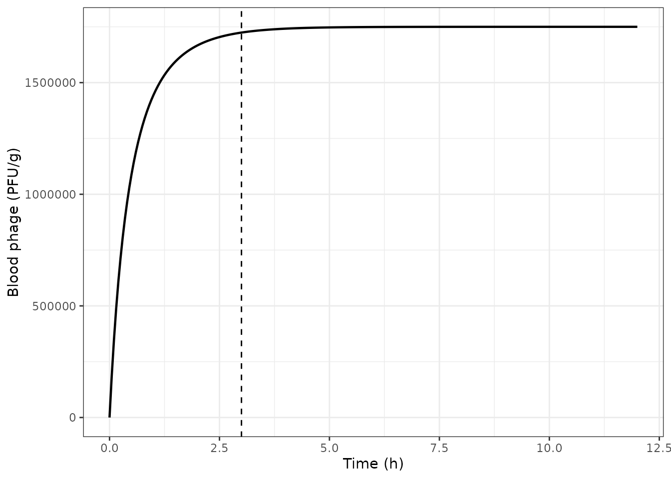
Continuous intravenous infusion in a 70 kg human: approach to steady state.
Assumptions, deviations and errata
The fitted observable was co-generated with a twin
free-125I model that is not reproducible
This is the most important caveat and it conditions
everything else. The measured quantity was 125I
scintillation counts, which is labelled phage plus free label.
Methods states:
“A twin PBPK model was constructed to describe free
125Iproduced through either thermal deconjugation of phage (a relatively slow process) or through degradation by the MPS (a relatively fast process).”
That twin model is load-bearing for the fitted observable, but it is described only in prose. Its equations, compartment list and parameter table appear in no source:
- The supplement’s Equations section covers the phage model only. A full-text scan of the supplement returns zero occurrences of “iodin”, “thyroid”, “deconjug”, “twin” or “125”.
- The global sensitivity analysis (Table S4) nevertheless
exercises two of the twin model’s parameters –
T_GI,LabandT_Urine,Lab, free-label transit – which appear in no parameter table and have no reported values. Table S4 lists 14 parameters against Table 1’s 10; the other two extras (F_PQ,F_KP) are perturbation factors used only by the sensitivity analysis and are not states or estimated parameters of either model.
These model files therefore implement the phage-disposition system alone. The parameter set they carry was estimated jointly with the missing twin model, so it is conditional on it. Practically, this is why the reconstruction cannot reproduce the shape of the Figure 2 post-hoc fits: those fitted lines are non-monotone in blood, lung, muscle, bone and stomach, dipping to a nadir around 8-12 h and then rising and plateauing out to 72 h. The printed phage system contains no slowly-releasing species that can produce a rise, and no choice of its parameters produces one. A free-label pool that accumulates as phage is catabolised does.
This vignette therefore validates against the paper’s reported model-derived summary statistics (terminal half-life, mean residence times, stomach-contents recovery, and the human dose projections) and deliberately does not attempt to replicate Figure 2.
Table 1 is the final parameter set; the abstract and Results narrative are stale
The abstract, the Results narrative and Table 1 report mutually inconsistent values for six parameters, and the abstract additionally swaps which organ group gets the small partition coefficient:
| Parameter | Abstract | Results text | Table 1 (used here) |
|---|---|---|---|
| Kp,LunKid | 0.000138 | – | 0.395 |
| Kp,LvrSpnSto | 0.627 | – | 2.12e-4 |
| Kp,Crs | 0.220 | – | 0.934 |
| PS | – | 0.0227 | 4.27e-2 |
| CLActive | – | 0.0145 | 1.29e-2 |
| TMPS,deg | – | 0.0301 h | 4.37e-2 h |
Table 1 was adopted because it, and not the narrative set, reproduces the paper’s own reported outputs: the blood terminal half-life and the liver mean residence time, both checked above. The narrative set gives a blood half-life of roughly 3 h against a reported 10.3-12.0 h.
The PAML-31-1 arm does not reconcile
Table 1 reports CL_Active = 1.29e-2, a
covariate-adjusted CL_Active,PAML = 1.34e-3, and
theta_PAML31 = -1.94. No standard transform connects the
three: exp(-1.94) = 1.85e-3, not 1.34e-3, and Table 1’s own
two clearance rows are 9.63-fold apart while the prose claims “10.7-fold
lower”. (Note that 0.0145 / 10.7 = 1.36e-3 – the narrative’s
CL_Active is what reproduces the 10.7-fold claim, which is
further evidence that the narrative and Table 1 come from different
runs.)
These models take both clearances directly from Table
1 and never evaluate theta. That reproduces the
direction of the PAML-31-1 effect (higher exposure) but not its
magnitude, and it badly overshoots the terminal half-life: a 9.6-fold
lower clearance with an unchanged distribution volume implies a terminal
half-life near 90 h, whereas the paper reports 12.0 h for PAML-31-1 –
essentially the same as the other two phages, alongside a 5.5-fold
higher AUC. A 5.5-fold exposure increase at an unchanged half-life
requires a proportional reduction in volume as well as clearance, which
this model structure does not have. Treat the PAML-31-1 arm as
not reproduced.
Blood topology reconstructed from Figure 1
The supplement’s venous equation does not conserve mass – it debits
Q_Lun * C_Lun,v where mass balance requires
Q_Lun * C_V – and every organ equation is driven by an
arterial concentration C_a(t) for which no equation is ever
given. Figure 1 shows unambiguous venous and arterial columns, so the
two-pool
venous -> lung -> arterial -> organs -> venous
topology was reconstructed from it. The choice is not decision-changing:
a single-pool blood model moves every output reported here by less than
3%.
The venous/arterial volume split (f_venous = 0.8) is
not reported by Echterhof 2026. It is the convention of
the nanoparticle-PBPK framework lineage this model is built on (Table S3
citations 6-7; the same 0.8 appears in
Kutumova_2024_albuminNanoparticles_mouse_pbpk). It is
exposed as a fixed() parameter so it can be changed.
The GI-elimination equation is not printed
Figure 1 draws a “GI Elimination” box fed by active clearance from
the liver, stomach, small intestine and large intestine, and Table 1
estimates a gastric transit half-life for it, but the supplement prints
no equation for that compartment – only the urine
analogue in the Kidney block. The gut_lumen state here is
reconstructed by direct analogy with the printed urine equation. The
reconstruction recovers the reported 18.0 %ID stomach-contents recovery
to within the gate applied above, which is evidence the analogy is the
right one.
The brain carries no MPS pool
Figure 1 draws an MPS box for the brain, but the supplement’s brain
block prints only the vascular and interstitial equations, with no
uptake, release or degradation terms. The printed equations are
followed. Table S3’s brain phagocyte density M_Brn is
consequently unused and is not declared in the model files.
The MPS pathway is nearly inert in the mouse, by construction
The MPS carrying capacity is a fixed absolute number of phage
particles (10^3.81 PFU per 100,000 phagocytes). At the
mouse doses actually administered (10^10.1 to
10^11.9 PFU) the whole-body capacity works out to roughly
5e5 PFU, about 0.001% of the dose, so the MPS
pools saturate essentially instantly and contribute almost nothing to
mouse clearance – active surface clearance does nearly all of it.
That is not an artefact of this implementation; it is a property of
the published parameter set, and the paper’s own global sensitivity
analysis independently confirms it: CL_Active has a
first-order Sobol index of 0.907 while A_MPS,
T_MPS,up and T_MPS,deg are all within noise of
zero (Table S4). In the rat and human, where tabulated phagocyte
densities are one to two orders of magnitude higher, the same capacity
relation makes the MPS the dominant route – which is what
produces the very short projected human half-life, and in turn the
paper’s own finding of rapid human elimination.
A_MPS is converted from PFU to %ID by the administered
dose
Table 1 gives A_MPS in
log10(PFU / 1e5 cells) while the main text describes the
same quantity as %ID per 1e5 phagocytes. The
two are reconciled by the dose: the Interspecies scaling section states
that “to simulate PFU per milliliter, doses were parameterized in PFU,
and the untransformed macrophage capacity term was
utilized”, which implies the %ID-scale fit used a transformed
one. These models therefore compute
A_RES [%ID/1e5 cells] = 10^A_MPS * 100 / DOSE_PHAGE_PFU.
Three independent checks confirm this reading over the alternative
(treating 10^3.81 as being already in %ID): it reproduces
the reported blood terminal half-life, it reproduces the liver mean
residence time, and it reproduces the Table S4 sensitivity ranking. The
alternative reading makes the MPS an effectively unbounded sink, giving
a blood half-life of minutes.
Numerical note: do not clamp the uptake rate
The saturable uptake rate k_up,max * (1 - A_res/A_max)
must be coded exactly as printed. Wrapping it in max(0, .)
puts a derivative kink precisely at the operating point
A_res ~ A_max, which stalls the implicit solver – with the
clamp in place the PAML-31-1 arm fails to integrate at all. Unclamped,
the relation is self-correcting and every arm solves in a couple of
seconds.
Simulated plasma versus measured whole blood
The model’s blood space is plasma: Table S3 calls the fraction
F_V_Pla, its mouse value (0.029) is a plasma-like rather
than whole-blood fraction, and the clinical simulation section states
that phage was assumed not to distribute into the red-blood-cell space.
The observed %ID/g, by contrast, was counted in whole
blood. A constant plasma-to-whole-blood factor of roughly
(1 - Hct) between the two is the most likely reason the
simulated blood AUC here runs above the reported whole-blood NCA AUC,
and it is consistent with the simulated 1-minute concentration (28
%ID/g) against the reported peak of about 15 %ID/g. This is offered as
the likely explanation, not as an established fact – the paper does not
state a haematocrit correction. Note that the quantities gated on above
(terminal half-life, mean residence times, the steady-state fraction)
are all invariant to a constant scale factor, which is why they were
chosen.
Other defects noted in the source
- Figure 2’s legend says LUZ19; the abstract, Methods, Results and Table S1 all say Luz24.
- Table S3’s row
F_V_Spnis captioned “Fraction of BW as Lung” – a copy-paste label error; the row is the spleen. - The supplement’s small-intestine block closes with two equations
named for the spleen (
k_Spn,up,A_Spn,max); they are plainly meant to be the small intestine. - The skin and carcass blocks each define
dC_x,V/dttwice, the second being the interstitial equation mislabelled.
Naming
The per-organ phagocyte pool uses the already-registered
int_<organ> sub-compartment namespace, whose founding
example (Kutumova_2024_albuminNanoparticles_mouse_pbpk)
uses it for exactly this state – the internalised, phagocytosed
nanoparticle pool of a whole-body mononuclear-phagocyte-system PBPK. The
stomach organ was added to the
pbpkSubCompartmentRegex organ vocabulary, and
vp_stomach registered, both of which the compartment
register calls routine extensions. The GI-elimination state reuses the
registered gut_lumen canonical.