Busulfan plasma and saliva (Xu 2023)
Source:vignettes/articles/Xu_2023_busulfan.Rmd
Xu_2023_busulfan.RmdModel and source
- Citation: Xu B, Yang T, Zhou J, Zheng Y, Wang J, Liu Q, Li D, Zhang Y, Liu M, Wu X. Saliva as a noninvasive sampling matrix for therapeutic drug monitoring of intravenous busulfan in Chinese patients undergoing hematopoietic stem cell transplantation: A prospective population pharmacokinetic and simulation study. CPT Pharmacometrics Syst Pharmacol. 2023;12(9):1238-1249. doi:10.1002/psp4.13004
- Description: One-compartment intravenous population PK model for busulfan in Chinese adult and paediatric patients undergoing allogeneic hematopoietic stem cell transplantation (Xu 2023), fitted jointly to paired plasma and saliva concentrations collected after the first 2-hour infusion. Saliva is not a separate kinetic compartment: the salivary busulfan concentration is the central-compartment (plasma) concentration multiplied by an estimated saliva:plasma scale factor of 0.88, a structure the authors selected over a kinetically distinct saliva compartment (dOFV = -82.52). Clearance and the central volume of distribution both increase with body surface area (power exponents 0.99 and 1.03 referenced to the population median BSA of 1.69 m^2); the volume additionally decreases with alkaline phosphatase (power exponent -0.20 referenced to the median ALP of 74 U/L). Separate proportional residual errors apply to plasma (12.92%) and saliva (22.50%).
- Article: https://doi.org/10.1002/psp4.13004
Busulfan (BU) has a narrow therapeutic window and is routinely dose-individualised by therapeutic drug monitoring (TDM) of plasma exposure. Xu and colleagues asked whether saliva – a noninvasive matrix – could replace plasma for that purpose, and built the first population PK model of intravenous busulfan that describes plasma and salivary concentrations jointly.
The answer they arrived at is structurally simple: saliva does
not behave as a kinetically distinct compartment. A
one-compartment plasma model whose central concentration is multiplied
by a single estimated scale factor fit the paired data
substantially better (dOFV = -82.52) than a model that gave saliva its
own compartment with its own transfer and elimination rate constants.
The alternative structure was additionally rejected because its saliva
elimination rate constant k20 was estimated with an
unacceptable 87% RSE (Xu 2023, Discussion).
That is what the packaged model encodes: one ODE state
(central) and two observations, Cc (plasma)
and Csaliva = fsaliva * Cc.
Population
Sixty-six Chinese patients with hematologic malignancies (54 adults and 12 children aged 6-17 years) undergoing allogeneic hematopoietic stem cell transplantation were enrolled at Fujian Medical University Union Hospital between November 2020 and November 2021 (Xu 2023 Methods, “Subjects”). Median age was 42 years (range 6-63), median weight 60.70 kg (range 25-90), median height 160 cm (range 123-190), median body surface area 1.69 m^2 (range 0.92-2.14) and median alkaline phosphatase 74 IU/L (range 36-253); 46 of 66 patients (69.7%) were male (Xu 2023 Table 1).
All patients received intravenous busulfan 0.8 mg/kg – dosed on adjusted ideal body weight – every 6 h as a 2-hour infusion for 4 consecutive days, as part of one of four myeloablative conditioning regimens. Paired plasma and saliva samples were drawn just before (0 h) and at 0.5, 2, 2.5, 3, 4 and 6 h after the start of the first dose. Of 406 paired collections, 406 plasma and 387 saliva samples were analysable; 19 saliva samples fell below the lower limit of quantitation and were deleted by the M1 method (Xu 2023 Results).
The same information is available programmatically via the model’s
population metadata
(readModelDb("Xu_2023_busulfan")()$population).
Source trace
Every ini() entry in
inst/modeldb/specificDrugs/Xu_2023_busulfan.R carries an
in-file comment pointing at its origin. They are collected here for
review.
| Equation / parameter | Value | Source location |
|---|---|---|
lcl (theta_CL) |
8.24 L/h | Table 3, final model (RSE 3%; bootstrap 7.75-8.77) |
lvc (theta_Vd) |
29.70 L | Table 3, final model (RSE 2%; bootstrap 28.32-31.14) |
lfsaliva (theta_Scale-factor) |
0.88 | Table 3, final model (RSE 2%; bootstrap 0.84-0.91) |
e_bsa_cl (theta_BSA-CL) |
0.99 | Table 3, final model (RSE 12%; bootstrap 0.76-1.27) |
e_bsa_vc (theta_BSA-Vd) |
1.03 | Table 3, final model (RSE 10%; bootstrap 0.77-1.22) |
e_alp_vc (theta_ALP-Vd) |
-0.20 | Table 3, final model (RSE 26%; bootstrap -0.31 to -0.09) |
etalcl |
0.0472764 | Table 3 IIV_CL = 22.00%; omega^2 = log(0.22^2 + 1) |
etalvc |
0.0183272 | Table 3 IIV_Vd = 13.60%; omega^2 = log(0.136^2 + 1) |
propSd |
0.1292 | Table 3 epsilon_plasma = 12.92% (RSE 17%) |
propSd_Csaliva |
0.2250 | Table 3 epsilon_saliva = 22.50% (RSE 22%) |
CL = theta_CL * (BSA/1.69)^theta_BSA_CL * exp(eta) |
n/a | Table 3 footnote equation (first displayed equation below the footnote list) |
Vd = theta_Vd * (BSA/1.69)^theta_BSA_Vd * (ALP/74)^theta_ALP_Vd * exp(eta) |
n/a | Table 3 footnote equation (second displayed equation) |
bsa_ref = 1.69 m^2 |
1.69 | Table 1 population median BSA; appears as the normalisation constant in the Table 3 footnote equations |
alp_ref = 74 IU/L |
74 | Table 1 population median ALP; appears as the normalisation constant in the Table 3 footnote equation |
d/dt(central) = -kel * central |
n/a | Methods, “Population pharmacokinetic analysis”: one-compartment constant-rate-infusion structure, NONMEM ADVAN1 TRANS2 |
Csaliva = fsaliva * Cc |
n/a | Figure 1 conceptual model + Results, “PopPK model” (scale factor assigned to the plasma compartment) |
CL_i (L/h) = 8.24 * (BSA_i/1.69)^0.99 |
n/a | Equation 5 (Discussion, initial-dose calculator) |
Dose (mg) = AUC_target * CL_i |
n/a | Equation 6 (Discussion, initial-dose calculator) |
The paper’s Table 3 footnotes f and g are
mislabelled – they read “Residual intra-individual variability of CL”
and “… of Vd” for the rows named epsilon_plasma and
epsilon_saliva. The row names, and the Discussion (“The
residual error of plasma was lower than the saliva (12.92%
vs. 22.50%)”), make the intended meaning unambiguous: these are the
plasma and saliva residual errors, and that is how they are encoded.
Virtual cohort
Original observed data are not publicly available. The cohort below follows the design the authors used for their own simulation study (Xu 2023 Methods, “Simulations and evaluation of the predictability of the model”): a positively skewed distribution of BSA with a corresponding normal distribution of ALP, both truncated to the observed ranges in Table 1.
Two arms are simulated, 200 subjects each (the validation cap):
-
Single 2-h infusion – one dose, sampled to 24 h,
for
Cmax/Tmax/AUC0-inf/t1/2. -
Steady state (q6h x 16) – the 16-dose regimen the
authors simulated, sampled across the final dosing interval, to test
their stated identity that
AUCsswithin a dosing interval equalsAUC0-infafter dose one.
Doses come from the paper’s own published initial-dose calculator (Equations 5 and 6), so no dosing assumption is imported from outside the paper. The AUC target is 1200 umolmin/L, the midpoint of the EMA-recommended 900-1500 umolmin/L window quoted in the Introduction.
set.seed(20230913)

n_per_arm <- 200L

# Busulfan molecular weight, C6H14O6S2 = 246.30 g/mol. Needed only to express
# the paper's umol*min/L AUC target in the ug/mL * h units the model works in.
mw_bu <- 246.30
umol_min_L_per_ug_h_mL <- 1000 / mw_bu * 60   # 1 ug*h/mL = 243.6 umol*min/L

auc_target_umol_min_L <- 1200                                     # EMA 900-1500 midpoint
auc_target_ug_h_mL <- auc_target_umol_min_L / umol_min_L_per_ug_h_mL

rtrunc <- function(n, rfun, lower, upper, ...) {
  out <- rfun(n, ...)
  bad <- out < lower | out > upper
  while (any(bad)) {
    out[bad] <- rfun(sum(bad), ...)
    bad <- out < lower | out > upper
  }
  out
}

make_subjects <- function(n, id_offset = 0L) {
  tibble(
    id = id_offset + seq_len(n),
    # Positive-skew BSA, median 1.69 m^2, truncated to Table 1's 0.92-2.14 range
    BSA = rtrunc(n, rlnorm, lower = 0.92, upper = 2.14,
                 meanlog = log(1.69), sdlog = 0.20),
    # Normal ALP, mean 74 IU/L, truncated to Table 1's 36-253 range
    ALP = rtrunc(n, rnorm, lower = 36, upper = 253, mean = 74, sd = 30)
  ) |>
    mutate(
      # Equation 5: typical individual clearance from BSA
      cl_pred = 8.24 * (BSA / 1.69)^0.99,
      # Equation 6: initial dose for the target AUC
      dose_mg = auc_target_ug_h_mL * cl_pred
    )
}

# Arm A: single 2-h infusion
subj_sd <- make_subjects(n_per_arm, id_offset = 0L) |>
  mutate(treatment = "Single 2-h infusion")

times_sd <- c(0, 0.25, 0.5, 0.75, 1, 1.25, 1.5, 1.75, 2, 2.25, 2.5,
              3, 3.5, 4, 4.5, 5, 5.5, 6, 7, 8, 10, 12, 16, 20, 24)

dose_sd <- subj_sd |>
  mutate(time = 0, evid = 1L, amt = dose_mg, dur = 2,
         cmt = "central", dvid = NA_integer_)

obs_sd <- subj_sd |>
  tidyr::crossing(time = times_sd, dvid = c(1L, 2L)) |>
  mutate(evid = 0L, amt = NA_real_, dur = NA_real_, cmt = "central")

# Arm B: q6h x 16 (steady state), sampled over the final dosing interval
subj_ss <- make_subjects(n_per_arm, id_offset = n_per_arm) |>
  mutate(treatment = "Steady state (q6h x 16)")

dose_times_ss <- seq(0, by = 6, length.out = 16)   # last dose starts at 90 h
times_ss <- seq(90, 96, by = 0.25)

dose_ss <- subj_ss |>
  tidyr::crossing(time = dose_times_ss) |>
  mutate(evid = 1L, amt = dose_mg, dur = 2, cmt = "central", dvid = NA_integer_)

obs_ss <- subj_ss |>
  tidyr::crossing(time = times_ss, dvid = c(1L, 2L)) |>
  mutate(evid = 0L, amt = NA_real_, dur = NA_real_, cmt = "central")

ev_cols <- c("id", "treatment", "time", "evid", "amt", "dur", "cmt", "dvid",
             "BSA", "ALP", "dose_mg", "cl_pred")

events <- bind_rows(
  dose_sd[ev_cols], obs_sd[ev_cols],
  dose_ss[ev_cols], obs_ss[ev_cols]
) |>
  arrange(id, time, desc(evid))

# IDs must be disjoint across arms; duplicates silently merge into one subject.
stopifnot(
  length(intersect(subj_sd$id, subj_ss$id)) == 0L,
  dplyr::n_distinct(events$id) == 2L * n_per_arm
)
Simulation
rxSolve() is asked for both endpoints.
dvid = 1 rows return the plasma observation
(sim) and dvid = 2 rows the saliva
observation, each with its own proportional residual error applied;
Cc and Csaliva (the residual-free individual
predictions) come back on every row. useLinCmt = FALSE is
required because rxode2’s automatic ODE-to-linCmt()
conversion corrupts the dvid mapping for multi-endpoint
models.
rxSolve() occasionally drops a subset of subjects to
NA with no warning, so the solve is retried until the
cohort comes back complete and then asserted.
mod <- readModelDb("Xu_2023_busulfan")

solve_complete <- function(model, events, n_expected, tries = 5L) {
  for (i in seq_len(tries)) {
    out <- as.data.frame(rxode2::rxSolve(
      model, events = events,
      keep = c("treatment", "BSA", "ALP", "dose_mg", "cl_pred", "dvid"),
      useLinCmt = FALSE
    ))
    ok <- dplyr::n_distinct(out$id) == n_expected &&
      all(is.finite(out$Cc)) && max(out$Cc, na.rm = TRUE) > 0
    if (ok) return(out)
  }
  stop("rxSolve() did not return a complete cohort after ", tries, " attempts")
}

sim <- solve_complete(mod, events, n_expected = 2L * n_per_arm)
#> ℹ parameter labels from comments will be replaced by 'label()'

sim <- sim |>
  mutate(
    matrix = ifelse(dvid == 1L, "Plasma", "Saliva"),
    # `sim` carries the endpoint-appropriate residual error for that row
    conc_obs = sim,
    conc_ipred = ifelse(dvid == 1L, Cc, Csaliva)
  )

stopifnot(
  dplyr::n_distinct(sim$id) == 2L * n_per_arm,
  all(is.finite(sim$conc_ipred))
)
A typical-value (no between-subject variability) solve is used for
the structural checks below. zeroRe() alone is not
sufficient once a stochastic solve has run in the same session – rxode2
retains that solve’s omega and silently re-samples etas –
so omega = NA is passed explicitly and the result is
asserted to be covariate-determined.
typ_subject <- tibble(id = 1L, BSA = 1.69, ALP = 74) |>
  mutate(cl_pred = 8.24 * (BSA / 1.69)^0.99,
         dose_mg = auc_target_ug_h_mL * cl_pred)

typ_events <- bind_rows(
  typ_subject |>
    mutate(time = 0, evid = 1L, amt = dose_mg, dur = 2,
           cmt = "central", dvid = NA_integer_),
  typ_subject |>
    tidyr::crossing(time = seq(0, 24, by = 0.1), dvid = c(1L, 2L)) |>
    mutate(evid = 0L, amt = NA_real_, dur = NA_real_, cmt = "central")
) |>
  arrange(time, desc(evid))

typ <- as.data.frame(rxode2::rxSolve(
  rxode2::zeroRe(mod), events = typ_events,
  keep = c("BSA", "ALP", "dvid"), useLinCmt = FALSE, omega = NA
))
#> ℹ parameter labels from comments will be replaced by 'label()'

# Mechanical guard: with IIV zeroed, CL must be exactly the covariate prediction.
stopifnot(dplyr::n_distinct(round(typ$cl, 8)) == 1L)
stopifnot(isTRUE(all.equal(unique(typ$cl), typ_subject$cl_pred, tolerance = 1e-6)))
Replicate published figures
Figure 2 (saliva VPC) and Figure S5 (plasma VPC)
Figure 2 of Xu 2023 is the visual predictive check of the saliva model over the first dosing interval; Figure S5 is the plasma counterpart. Both are reproduced here as 5th / 50th / 95th percentiles of the simulated observations (individual prediction plus proportional residual error) for the single-dose arm.
sim |>
  filter(treatment == "Single 2-h infusion", time <= 6) |>
  group_by(matrix, time) |>
  summarise(
    Q05 = quantile(conc_obs, 0.05, na.rm = TRUE),
    Q50 = quantile(conc_obs, 0.50, na.rm = TRUE),
    Q95 = quantile(conc_obs, 0.95, na.rm = TRUE),
    .groups = "drop"
  ) |>
  ggplot(aes(time, Q50)) +
  geom_ribbon(aes(ymin = Q05, ymax = Q95), alpha = 0.25, fill = "steelblue") +
  geom_line(linewidth = 0.8) +
  facet_wrap(~matrix) +
  labs(
    x = "Time after start of the first infusion (h)",
    y = "Busulfan concentration (ug/mL)",
    title = "Simulated 5th / 50th / 95th percentiles over the first dosing interval",
    caption = "Replicates Figure 2 (saliva) and Figure S5 (plasma) of Xu 2023."
  )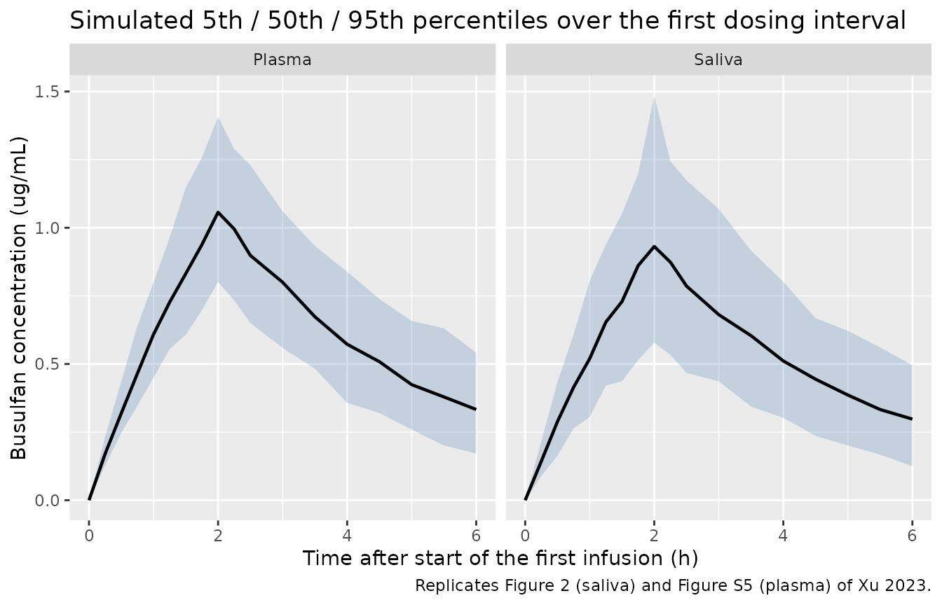
Figure 1 (conceptual model): the scale factor is time-invariant
Figure 1 draws saliva as the central compartment rescaled, not as a
compartment with its own kinetics. The consequence is that the
individual-prediction saliva / plasma ratio is exactly
fsaliva at every time, for every subject and every
covariate combination – there is no distribution delay and no separate
terminal slope. That is asserted rather than merely plotted.
ratio_ipred <- typ |>
  filter(time > 0) |>
  transmute(ratio = Csaliva / Cc) |>
  pull(ratio)

stopifnot(isTRUE(all.equal(range(ratio_ipred), c(0.88, 0.88), tolerance = 1e-8)))

typ |>
  filter(dvid == 1L) |>
  select(time, Plasma = Cc, Saliva = Csaliva) |>
  tidyr::pivot_longer(-time, names_to = "matrix", values_to = "conc") |>
  ggplot(aes(time, conc, colour = matrix)) +
  geom_line(linewidth = 0.8) +
  scale_y_log10() +
  labs(
    x = "Time (h)", y = "Busulfan concentration (ug/mL)", colour = NULL,
    title = "Typical-value profile, BSA 1.69 m^2 and ALP 74 IU/L",
    caption = paste(
      "Replicates the structure of Figure 1 of Xu 2023: saliva is the central",
      "compartment scaled by 0.88, so the two curves are parallel on the log scale."
    )
  )
#> Warning in scale_y_log10(): log-10 transformation introduced infinite values.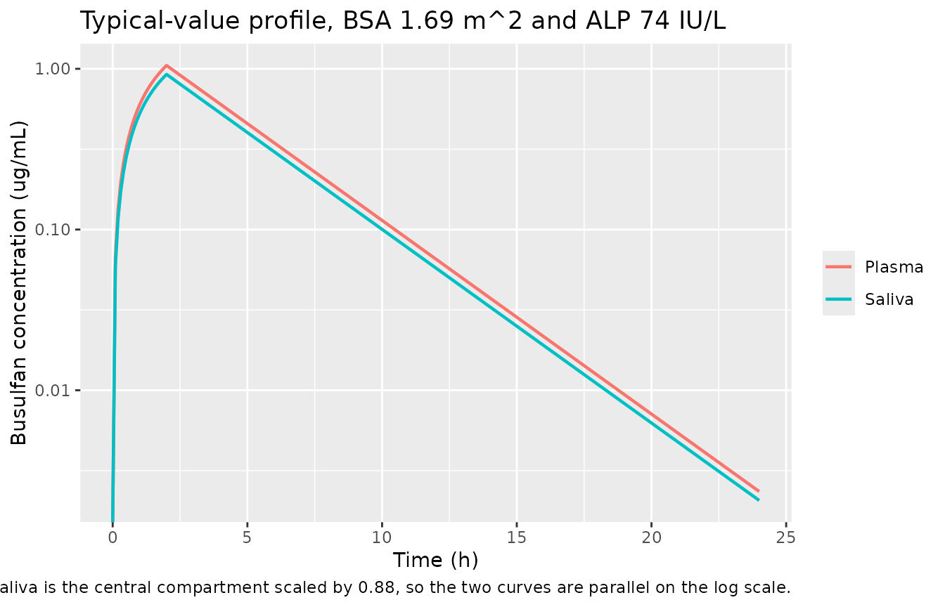
Table 2: saliva / plasma ratio and concentration-time profile
Table 2 of Xu 2023 reports, at each sampling time, the mean +/- SD
plasma concentration, saliva concentration, and saliva/plasma (S/P)
ratio in the observed data. The S/P ratio is the sharpest available
check on this model, because its central tendency is set by
fsaliva alone and its spread is set by the two
residual-error terms alone:
SD(S/P) ~ fsaliva * sqrt(propSd^2 + propSd_Csaliva^2).
paper_times <- c(0.5, 1.0, 1.5, 2.0, 2.5, 3, 4, 5, 6)

published_t2 <- tibble::tribble(
  ~time, ~plasma_ref, ~saliva_ref, ~sp_ref, ~sp_ref_sd,
  0.5,   0.59,        0.53,        0.90,    0.12,
  1.0,   0.71,        0.61,        0.87,    0.14,
  1.5,   0.98,        0.88,        0.88,    0.21,
  2.0,   1.16,        0.99,        0.88,    0.22,
  2.5,   1.00,        0.91,        0.92,    0.24,
  3.0,   0.89,        0.74,        0.85,    0.19,
  4.0,   0.69,        0.60,        0.89,    0.24,
  5.0,   0.58,        0.50,        0.89,    0.32,
  6.0,   0.42,        0.37,        0.90,    0.20
)

sim_t2 <- sim |>
  filter(treatment == "Single 2-h infusion", time %in% paper_times) |>
  select(id, time, matrix, conc_obs) |>
  tidyr::pivot_wider(names_from = matrix, values_from = conc_obs) |>
  mutate(sp = Saliva / Plasma) |>
  group_by(time) |>
  summarise(
    plasma_sim = mean(Plasma),
    saliva_sim = mean(Saliva),
    sp_sim = mean(sp),
    sp_sim_sd = sd(sp),
    .groups = "drop"
  )

t2 <- published_t2 |>
  left_join(sim_t2, by = "time") |>
  mutate(
    plasma_pct = 100 * (plasma_sim - plasma_ref) / plasma_ref,
    saliva_pct = 100 * (saliva_sim - saliva_ref) / saliva_ref,
    sp_pct = 100 * (sp_sim - sp_ref) / sp_ref
  )

t2 |>
  transmute(
    `Time (h)` = time,
    `Plasma, observed (ug/mL)` = round(plasma_ref, 2),
    `Plasma, simulated (ug/mL)` = round(plasma_sim, 2),
    `Plasma % diff` = round(plasma_pct, 1),
    `Saliva, observed (ug/mL)` = round(saliva_ref, 2),
    `Saliva, simulated (ug/mL)` = round(saliva_sim, 2),
    `Saliva % diff` = round(saliva_pct, 1)
  ) |>
  knitr::kable(
    caption = paste(
      "Replicates Table 2 of Xu 2023 (mean concentrations by sampling time).",
      "Observed values are the paper's; simulated values are cohort means of the",
      "residual-error-included simulated observations."
    )
)| Time (h) | Plasma, observed (ug/mL) | Plasma, simulated (ug/mL) | Plasma % diff | Saliva, observed (ug/mL) | Saliva, simulated (ug/mL) | Saliva % diff |
|---|---|---|---|---|---|---|
| 0.5 | 0.59 | 0.33 | -43.8 | 0.53 | 0.29 | -44.6 |
| 1.0 | 0.71 | 0.61 | -13.5 | 0.61 | 0.53 | -13.2 |
| 1.5 | 0.98 | 0.85 | -13.2 | 0.88 | 0.74 | -15.7 |
| 2.0 | 1.16 | 1.07 | -7.6 | 0.99 | 0.96 | -2.7 |
| 2.5 | 1.00 | 0.92 | -8.2 | 0.91 | 0.81 | -11.5 |
| 3.0 | 0.89 | 0.80 | -10.4 | 0.74 | 0.71 | -4.0 |
| 4.0 | 0.69 | 0.58 | -15.6 | 0.60 | 0.53 | -12.3 |
| 5.0 | 0.58 | 0.44 | -24.0 | 0.50 | 0.39 | -21.1 |
| 6.0 | 0.42 | 0.34 | -19.1 | 0.37 | 0.30 | -18.4 |
t2 |>
  transmute(
    `Time (h)` = time,
    `S/P observed (mean)` = round(sp_ref, 2),
    `S/P observed (SD)` = round(sp_ref_sd, 2),
    `S/P simulated (mean)` = round(sp_sim, 2),
    `S/P simulated (SD)` = round(sp_sim_sd, 2),
    `% diff (mean)` = round(sp_pct, 1)
  ) |>
  knitr::kable(
    caption = paste(
      "Saliva/plasma ratio, replicating the S/P columns of Table 2 of Xu 2023.",
      "The paper reports an overall S/P of 0.89 +/- 0.22."
    )
)| Time (h) | S/P observed (mean) | S/P observed (SD) | S/P simulated (mean) | S/P simulated (SD) | % diff (mean) |
|---|---|---|---|---|---|
| 0.5 | 0.90 | 0.12 | 0.90 | 0.25 | 0.0 |
| 1.0 | 0.87 | 0.14 | 0.88 | 0.26 | 1.1 |
| 1.5 | 0.88 | 0.21 | 0.89 | 0.22 | 1.3 |
| 2.0 | 0.88 | 0.22 | 0.91 | 0.24 | 3.7 |
| 2.5 | 0.92 | 0.24 | 0.90 | 0.26 | -2.3 |
| 3.0 | 0.85 | 0.19 | 0.91 | 0.24 | 6.8 |
| 4.0 | 0.89 | 0.24 | 0.92 | 0.25 | 3.8 |
| 5.0 | 0.89 | 0.32 | 0.92 | 0.25 | 2.8 |
| 6.0 | 0.90 | 0.20 | 0.91 | 0.25 | 0.7 |
sp_overall <- sim |>
  filter(treatment == "Single 2-h infusion", time %in% paper_times) |>
  select(id, time, matrix, conc_obs) |>
  tidyr::pivot_wider(names_from = matrix, values_from = conc_obs) |>
  mutate(sp = Saliva / Plasma) |>
  summarise(mean = mean(sp), sd = sd(sp))

sp_theory <- 0.88 * sqrt(0.1292^2 + 0.2250^2)
Pooled across the paper’s sampling times the simulated S/P ratio is
0.90 +/- 0.25, against the paper’s observed 0.89 +/- 0.22.
The closed-form spread implied by the two residual errors,
0.88 * sqrt(0.1292^2 + 0.2250^2), is 0.228 – so the pooled
observed variability in the S/P ratio is accounted for by the model’s
residual-error structure alone, with no between-subject variability on
the scale factor required. (Per timepoint the agreement is looser in
both directions: the paper’s observed S/P SDs span 0.12-0.32 across the
nine sampling times against a simulated 0.22-0.26, on observed subsets
as small as n = 9.) That is consistent with the authors’ own finding
that the shrinkage on the scale-factor IIV reached 100%, so the term had
to be dropped.
Dose-scale diagnostic for the absolute concentration level
The simulated concentrations in the table above sit below the observed means at every timepoint. That is expected and is quantified here rather than asserted: the trial dosed 0.8 mg/kg on adjusted ideal body weight, which needs per-subject height and sex (not reported), so this vignette instead doses each virtual subject from the paper’s own Equation 5-6 calculator at the 1200 umol*min/L target. In a linear one-compartment model concentration is proportional to dose, so a pure dose mismatch appears as one common multiplicative offset. The post-infusion rows (t >= 2 h, after the 2-hour infusion has ended) are the ones free of infusion-timing artefacts.
offset <- t2 |>
  mutate(
    ratio_plasma = plasma_sim / plasma_ref,
    ratio_saliva = saliva_sim / saliva_ref,
    phase = ifelse(time >= 2, "Post-infusion", "Intra-infusion")
  )

offset_post <- offset |> filter(time >= 2)
ratios_post <- c(offset_post$ratio_plasma, offset_post$ratio_saliva)

# One common dose-scale factor implied by the post-infusion rows of both matrices
implied_dose_ratio <- exp(mean(log(ratios_post)))
implied_dose_excess_pct <- 100 * (1 / implied_dose_ratio - 1)
shortfall_post_pct <- range(100 * (1 - ratios_post))
shortfall_intra_pct <- range(100 * (1 - c(offset$ratio_plasma[offset$time < 2],
                                          offset$ratio_saliva[offset$time < 2])))

# A single constant offset would leave the ratio flat in time. Quantify the drift
# by the apparent 2 -> 6 h decline half-life of each mean series.
decline_hl <- function(c2, c6) 4 * log(2) / log(c2 / c6)
hl_obs_plasma <- decline_hl(t2$plasma_ref[t2$time == 2], t2$plasma_ref[t2$time == 6])
hl_sim_plasma <- decline_hl(t2$plasma_sim[t2$time == 2], t2$plasma_sim[t2$time == 6])

offset |>
  transmute(
    `Time (h)` = time,
    Phase = phase,
    `Plasma sim/obs` = round(ratio_plasma, 3),
    `Saliva sim/obs` = round(ratio_saliva, 3)
  ) |>
  knitr::kable(
    caption = paste(
      "Simulated/observed mean-concentration ratio by sampling time.",
      "A pure dose-scale mismatch would hold this ratio constant."
    )
)| Time (h) | Phase | Plasma sim/obs | Saliva sim/obs |
|---|---|---|---|
| 0.5 | Intra-infusion | 0.562 | 0.554 |
| 1.0 | Intra-infusion | 0.865 | 0.868 |
| 1.5 | Intra-infusion | 0.868 | 0.843 |
| 2.0 | Post-infusion | 0.924 | 0.973 |
| 2.5 | Post-infusion | 0.918 | 0.885 |
| 3.0 | Post-infusion | 0.896 | 0.960 |
| 4.0 | Post-infusion | 0.844 | 0.877 |
| 5.0 | Post-infusion | 0.760 | 0.789 |
| 6.0 | Post-infusion | 0.809 | 0.816 |
Over the post-infusion rows the simulated means run 2.7-24.0% below the observed ones, and a single dose-scale factor of 0.868 accounts for the bulk of that – i.e. the trial’s realised adjusted-ideal-body-weight doses averaged about 15% higher than the calculator returns at the 1200 umol*min/L target, which is the midpoint of the EMA 900-1500 window.
The ratio is not perfectly flat, so the offset is not purely dose-scale: in plasma it drifts from 0.92 at 2 h to 0.81 at 6 h. The apparent 2-to-6 h decline half-life is 2.41 h simulated against 2.73 h for the observed means – both inside the 2-3 h terminal half-life the paper quotes for busulfan (Introduction). The observed means are cross-sectional over different and unequal subject subsets at each time (n = 9-70 in Table 2), so this is weak evidence about shape in either direction.
PKNCA validation
NCA is run separately for each matrix, with the two arms carried as the treatment grouping and arm-specific intervals.
nca_conc <- function(matrix_name) {
  sim |>
    filter(treatment == "Single 2-h infusion", matrix == matrix_name) |>
    filter(!is.na(conc_obs)) |>
    select(id, time, treatment, Cc = conc_obs)
}

nca_dose <- events |>
  filter(evid == 1, treatment == "Single 2-h infusion") |>
  select(id, time, amt, treatment)

intervals_sd <- data.frame(
  start = 0, end = Inf,
  cmax = TRUE, tmax = TRUE, aucinf.obs = TRUE, half.life = TRUE
)

run_nca_sd <- function(matrix_name) {
  conc_obj <- PKNCA::PKNCAconc(nca_conc(matrix_name), Cc ~ time | treatment + id)
  dose_obj <- PKNCA::PKNCAdose(
    nca_dose, amt ~ time | treatment + id,
    route = "intravascular", duration = 2
  )
  res <- PKNCA::pk.nca(
    PKNCA::PKNCAdata(conc_obj, dose_obj, intervals = intervals_sd)
  )
  as.data.frame(res) |>
    mutate(matrix = matrix_name)
}

nca_sd <- bind_rows(run_nca_sd("Plasma"), run_nca_sd("Saliva"))
Comparison against published values
The paper does not tabulate NCA parameters for its own dataset, so the reference column is assembled from the values it does report:
- Cmax – the 2 h row of Table 2 (1.16 ug/mL plasma, 0.99 ug/mL saliva); the Results state “The BU peak in both matrices appeared at 2 h after administration”, which is the end of the 2-hour infusion.
- Tmax – 2 h, from the same sentence.
- t1/2 – 2.5 h, the midpoint of the “terminal half-life of 2-3 h” quoted in the Introduction (Xu 2023 reference 11) as the accepted busulfan value.
-
AUC0-inf – the 1200 umolmin/L design target
used to compute each subject’s dose via Equations 5-6, converted to mass
units (4.926 ugh/mL), and multiplied by 0.88 for saliva. This row
is a structural identity check – numerically integrated
AUC against
Dose / CL– not an independent validation.
published_nca <- tibble::tribble(
  ~matrix,   ~cmax, ~tmax, ~aucinf.obs,                 ~half.life,
  "Plasma",  1.16,  2.0,   auc_target_ug_h_mL,          2.5,
  "Saliva",  0.99,  2.0,   auc_target_ug_h_mL * 0.88,   2.5
)

cmp <- nlmixr2lib::ncaComparisonTable(
  simulated = nca_sd,
  reference = published_nca,
  by = "matrix",
  units = c(cmax = "ug/mL", tmax = "h",
            aucinf.obs = "ug*h/mL", half.life = "h"),
  tolerance_pct = 20
)

knitr::kable(
  cmp,
  caption = "Simulated vs. published/derived NCA. * differs from reference by >20%.",
  align = c("l", "l", "r", "r", "r")
)| NCA parameter | matrix | Reference | Simulated | % diff |
|---|---|---|---|---|
| Cmax (ug/mL) | Plasma | 1.16 | 1.12 | -3.5% |
| Cmax (ug/mL) | Saliva | 0.99 | 1.08 | +9.1% |
| Tmax (h) | Plasma | 2 | 2 | +0.0% |
| Tmax (h) | Saliva | 2 | 2 | +0.0% |
| AUC0-∞ (obs) (ug*h/mL) | Plasma | 4.93 | 4.86 | -1.3% |
| AUC0-∞ (obs) (ug*h/mL) | Saliva | 4.33 | 4.3 | -0.8% |
| t½ (h) | Plasma | 2.5 | 2.41 | -3.5% |
| t½ (h) | Saliva | 2.5 | 2.39 | -4.5% |
attr(cmp, "footnote")
#> NULL
Steady state: AUCss within a dosing interval equals AUC0-inf after dose one
The authors’ simulation study rests on the identity “The AUCss within
each dose interval is equal to the AUC0-inf after dose one” (Xu 2023
Discussion), which they use to justify validating AUCss
prediction against a single-dose calculation. For a linear
one-compartment model this is exact, and it is checked here against the
simulated q6h x 16 arm.
intervals_ss <- data.frame(start = 90, end = 96, auclast = TRUE)

run_nca_ss <- function(matrix_name) {
  ss_conc <- sim |>
    filter(treatment == "Steady state (q6h x 16)", matrix == matrix_name) |>
    filter(!is.na(conc_ipred)) |>
    select(id, time, treatment, Cc = conc_ipred)
  conc_obj <- PKNCA::PKNCAconc(ss_conc, Cc ~ time | treatment + id)
  res <- PKNCA::pk.nca(PKNCA::PKNCAdata(conc_obj, intervals = intervals_ss))
  as.data.frame(res) |>
    filter(PPTESTCD == "auclast") |>
    transmute(id, matrix = matrix_name, auc_ss = PPORRES)
}

auc_ss <- bind_rows(run_nca_ss("Plasma"), run_nca_ss("Saliva"))
#> No dose information provided, calculations requiring dose will return NA.
#> No dose information provided, calculations requiring dose will return NA.

# Closed-form AUCss = Dose / CL_i (x 0.88 for saliva), using each subject's
# realised individual clearance from the simulation.
cl_indiv <- sim |>
  filter(treatment == "Steady state (q6h x 16)") |>
  distinct(id, dose_mg, cl) |>
  mutate(auc_closed_plasma = dose_mg / cl)

ss_check <- auc_ss |>
  left_join(cl_indiv, by = "id") |>
  mutate(
    auc_closed = ifelse(matrix == "Plasma",
                        auc_closed_plasma, auc_closed_plasma * 0.88),
    pct_diff = 100 * (auc_ss - auc_closed) / auc_closed
  )

ss_check |>
  group_by(matrix) |>
  summarise(
    `AUCss, numerically integrated (ug*h/mL)` = round(median(auc_ss), 3),
    `AUCss = Dose/CL closed form (ug*h/mL)` = round(median(auc_closed), 3),
    `Median % difference` = round(median(pct_diff), 2),
    `Max |% difference|` = round(max(abs(pct_diff)), 2),
    .groups = "drop"
  ) |>
  dplyr::rename(Matrix = matrix) |>
  knitr::kable(
    caption = paste(
      "Steady-state identity check over the 16th dosing interval (90-96 h).",
      "Confirms AUCss within a dosing interval equals Dose/CL, the assumption",
      "underlying the authors' simulation study."
    )
)| Matrix | AUCss, numerically integrated (ug*h/mL) | AUCss = Dose/CL closed form (ug*h/mL) | Median % difference | Max |% difference| |
|---|---|---|---|---|
| Plasma | 4.871 | 4.872 | -0.03 | 0.17 |
| Saliva | 4.287 | 4.288 | -0.03 | 0.17 |
Assumptions and deviations
-
Dosing. The paper’s patients received 0.8 mg/kg on
adjusted ideal body weight, which requires per-subject
height and sex; neither is reported at the subject level. Virtual
subjects are therefore dosed with the paper’s own published initial-dose
calculator (Equations 5 and 6:
CL_i = 8.24 * (BSA_i/1.69)^0.99,Dose = AUC_target * CL_i) at the midpoint of the EMA 900-1500 umol*min/L target window. Every input to that calculation comes from the paper. - Molecular weight. Converting the paper’s umolmin/L AUC targets into the ug/mL h units the model works in requires busulfan’s molecular weight, 246.30 g/mol (C6H14O6S2). This is a physical constant, not a model parameter, and is the only number in this vignette that is not from Xu 2023.
- Covariate distributions. BSA is drawn log-normally (median 1.69 m^2, sdlog 0.20) and ALP normally (mean 74 IU/L, SD 30) and both are truncated to the Table 1 ranges. This follows the authors’ stated simulation design (“a positive skew distribution of BSA and corresponding normal distribution of ALP”) but the dispersion parameters themselves are not reported; only the medians and ranges are. Marginal quantiles of the drawn cohort therefore need not match the unreported observed distribution.
- Absolute concentration level. Simulated mean concentrations sit 2.7-24.0% below the Table 2 observed means over the post-infusion timepoints, and 13.2-44.6% below them intra-infusion. This is predominantly a dose-scale offset rather than a structural mismatch: concentrations in a linear one-compartment model are proportional to dose, and the simulated doses come from the paper’s Equation 5-6 calculator at the 1200 umol*min/L target rather than from the 0.8 mg/kg adjusted-ideal-body-weight doses the patients actually received (which are not reported per subject). One common dose-scale factor of 0.868 – realised doses about 15% above the calculator’s – accounts for the bulk of it; the residual drift in that ratio with time is quantified in the dose-scale diagnostic above and is not resolvable from the reported data. The dose-independent checks – the S/P ratio at every timepoint, Tmax, and t1/2 – match the paper closely, which is the intended reading of these tables.
- Intra-infusion timepoints. The 0.5 h row is the largest single deviation (-43.8% plasma and -44.6% saliva). Table 2 bins actual sampling times, and its early bins are very sparse (n = 14, 16 and 9 at 0.5, 1.0 and 1.5 h, against 58-70 at 2-3 h) for a protocol whose only nominal intra-infusion sample was at 0.5 h; the simulation assumes every infusion ran exactly 2 h at a constant rate. Neither the realised infusion durations nor the actual sample times are reported, so this cannot be resolved from the available sources. It does not affect the model’s own VPC (Figure 2), which the authors report as satisfactory.
- Cmax on noisy simulated data. PKNCA takes Cmax as the maximum over the sampling grid, so proportional residual error biases it upward relative to the mean concentration at the true peak time. The effect is larger for saliva (22.50% residual) than for plasma (12.92%), which is why simulated saliva Cmax sits above its reference while simulated plasma Cmax sits below. Both remain well inside the 20% flagging tolerance.
-
IIV convention. Table 3 reports IIV as a bare
percentage on an exponential error model with no stated convention. It
is encoded here as a CV%, i.e.
omega^2 = log(CV^2 + 1). The alternative reading (percentage = omega x 100) would give 0.0484 and 0.0185 instead of 0.0473 and 0.0183 – a difference of under 2.5% in variance, with no visible effect on any output in this vignette. -
Saliva scale factor has no IIV. The authors
estimated IIV on the scale factor, found 100% shrinkage, and dropped it
(Xu 2023 Discussion, limitations). The packaged model reproduces that:
fsalivais a fixed-effect-only parameter, so all saliva/plasma variability is residual. - Base model not packaged. Table 3 also reports a covariate-free base model (CL 7.89 L/h, Vd 28.30 L, scale factor 0.88, IIV 28.20% / 27.50%). Only the final model is packaged, per the library’s convention of shipping the author’s final model.
-
Rejected alternative structure not packaged. The
Discussion reports the rejected separate-saliva-compartment model (CL
6.22 L/h, k12 0.074 /h, k20 10 /h). It was rejected by the authors on
OFV and on an 87% RSE for
k20, so it is not packaged. - Supplement not available. Tables S1 (example data file) and S2 (NONMEM model code) and Figures S1-S8 are referenced but were not available when this model was built. Every parameter value and every equation encoded in the model file comes from the main article’s Table 3 and its footnote equations, so the supplement is not needed for the extraction; it would only have provided an independent cross-check of the control stream.
-
Naming. The saliva:plasma scale factor is encoded
as
lfsaliva/fsaliva, and the saliva observation asCsaliva, following thef<matrix>/C<matrix>pattern established byLandersdorfer_2009_moxifloxacin.R(lfcortical/fcortical/Ccorticalfor the bone:serum equilibrium concentration ratio).