Sipoglitazar (Stringer 2013)
Source:vignettes/articles/Stringer_2013_sipoglitazar.Rmd
Stringer_2013_sipoglitazar.RmdModel and source
Stringer 2013 fits two population PK models to the same pooled data set, and both are packaged here:
uiGeno <- rxode2::rxode(readModelDb("Stringer_2013_sipoglitazar"))
#> ℹ parameter labels from comments will be replaced by 'label()'
#> Warning: some etas defaulted to non-mu referenced, possible parsing error: etapropSdPhase2
#> as a work-around try putting the mu-referenced expression on a simple line
uiMix  <- rxode2::rxode(readModelDb("Stringer_2013_sipoglitazar_mixture"))
#> ℹ parameter labels from comments will be replaced by 'label()'
#> Warning: some etas defaulted to non-mu referenced, possible parsing error: etapropSdPhase2
#> as a work-around try putting the mu-referenced expression on a simple line- Citation: Stringer F, Ploeger BA, DeJongh J, Scott G, Urquhart R, Karim A, Danhof M. Evaluation of the Impact of UGT Polymorphism on the Pharmacokinetics and Pharmacodynamics of the Novel PPAR Agonist Sipoglitazar. J Clin Pharmacol. 2013;53(3):256-263. doi:10.1177/0091270012447121.
-
Stringer_2013_sipoglitazar: Two-compartment population PK model for sipoglitazar with UGT2B15 genotype-stratified apparent clearance in healthy volunteers and adults with type 2 diabetes -
Stringer_2013_sipoglitazar_mixture: Two-compartment population PK model for sipoglitazar with apparent clearance assigned to one of three latent metabolizer subpopulations by a NONMEM mixture model, fitted without using UGT2B15 genotype - Article: https://doi.org/10.1177/0091270012447121
- Supplement: supplementary online material at the journal (Table A1, Figures S1-S4)
Sipoglitazar is an investigational oral PPAR alpha / delta / gamma
agonist that is cleared by UGT-catalysed glucuronidation. The
UGT2B15 D85Y (*2) allele reduces that activity,
and the paper’s question is how far the genotype explains the wide
spread in clearance seen in phase I.
The genotype model assigns each subject’s typical
clearance from the observed UGT2B15 genotype. The
mixture model was fitted in parallel, with the NONMEM
$MIX subroutine assigning each subject to one of three
latent metabolizer subpopulations from apparent clearance
alone, deliberately ignoring the genotype. Everything else about the two
models is the same. Comparing them is the paper’s central argument: 61
of the 744 subjects genotyped *1/*1 or *1/*2
(8%) are placed in the poor-metaboliser subpopulation by the mixture
model, i.e. their phenotype does not follow their genotype.
Population
The analysis pools 1151 subjects from 3 studies (Stringer 2013 Table 1):
- Phase I study 006 – 524 healthy volunteers (304 female), median age 26 years (18-55), median weight 71 kg (48-113). A single oral 64 mg dose with dense sampling at 0, 1, 2, 3, 4, 6, 8, 12, 16 and 24 h.
- Phase II study EC201 – 320 adults with type 2 diabetes and no prior antidiabetic medication (155 female), median age 56 years (34-75), median weight 90 kg (60-149). Placebo and 8, 16, 32 and 64 mg daily for 12 weeks.
- Phase II study EC202 – 307 adults with type 2 diabetes (164 female), median age 57 years (34-74), median weight 87 kg (55-149). Placebo and 32 or 64 mg total daily dose, once or twice daily, for 12 weeks.
Pooled UGT2B15 genotype frequencies were
*1/*1 22%, *1/*2 51% and *2/*2
27%. The phase II studies contributed three trough samples per subject
(weeks 4, 6 and 8) whose actual time after dose was never recorded,
which is why the model carries a separate – and much larger, and itself
variable – residual error for that stratum.
The same information is available programmatically via
readModelDb("Stringer_2013_sipoglitazar")()$population.
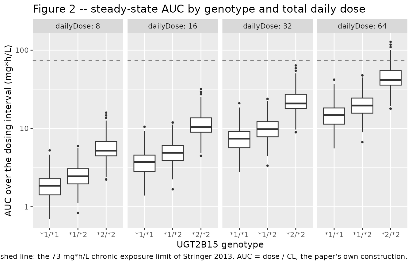
A predetermined chronic-exposure safety limit of AUC > 73 mg*h/L is quoted in Methods and drawn as a grey line on Figure 2; it is used below.
Source trace
Per-parameter origins are recorded as in-file comments next to each
ini() entry in
inst/modeldb/specificDrugs/Stringer_2013_sipoglitazar.R and
..._mixture.R. Collected here for review.
| Equation / parameter | Genotype model | Mixture model | Source location |
|---|---|---|---|
| Structural model | 2-compartment, zero-order input into a depot then first-order absorption, linear elimination | same | Results, Base Model; Methods, Population Data Analysis |
lcl_s1s1 / lcl_em
|
4.46 L/h | 5.04 L/h | Table 2 / Suppl. Table A1, CL (*1/*1) /
CL POP1 (EM)
|
lcl_s1s2 / lcl_im
|
3.25 L/h | 3.35 L/h | Table 2 / Suppl. Table A1, CL (*1/*2) /
CL POP2 (IM)
|
lcl_s2s2 / lcl_pm
|
1.53 L/h | 1.53 L/h | Table 2 / Suppl. Table A1, CL (*2/*2) /
CL POP3 (PM)
|
lvc |
9.03 L | 9.06 L | Table 2 / Suppl. Table A1, V
|
lvp |
1.71 L | 0.188 x 9.06 = 1.703 L | Table 2 / Suppl. Table A1, V2 and footnote b |
lq |
0.313 L/h | 0.311 L/h | Table 2 / Suppl. Table A1, Q
|
lka |
2.07 1/h | 2.15 1/h | Table 2 / Suppl. Table A1, ka / ka1
|
ld1 |
0.568 h | 0.637 h | Table 2 / Suppl. Table A1, D1
|
e_ffm_vc |
0.00349 1/kg | 0.00556 1/kg | Table 2 / Suppl. Table A1, theta(f); form from equation
4 |
| Covariate equation | P = theta(i) * (1 + theta(f) * (COV - COV_median)) |
same | Equation 4, p. 258 |
| IIV form | theta_i = theta_mean * exp(eta_i) |
same | Equation 1, p. 258 |
etalcl |
40.25% CV | 38.21% CV | Table 2 / Suppl. Table A1, IIV column |
etalvc |
34.21% CV | 34.50% CV | Table 2 / Suppl. Table A1, IIV column |
etald1 |
78.29% CV | 77.20% CV | Table 2 / Suppl. Table A1, IIV column |
propSdPhase1 |
sqrt(0.0552) = 0.2349 | sqrt(0.05487) = 0.2342 | Table 2 / Suppl. Table A1, residual phase I |
propSdPhase2 |
sqrt(0.167) = 0.4087 | sqrt(0.167) = 0.4087 | Table 2 / Suppl. Table A1, residual phase II |
etapropSdPhase2 |
76.88% CV | 72.18% CV | Table 2 / Suppl. Table A1, IIV on the phase II residual |
| Residual form |
C = PRED * (1 + ERR) (phase I),
C = PRED * (1 + ERR) with IIV on ERR (phase II) |
same | Equations 2 and 3, p. 258-259 |
| Mixture weights | n/a | POP1 0.18, POP2 0.522, POP3 0.30 | Suppl. Table A1,
Probability of belonging to POP 1/2/3
|
| Exposure limit 73 mg*h/L | n/a | n/a | Methods, Population Data Analysis; Figure 2 grey line |
Virtual cohort
Original observed data are not publicly available. The cohort below
reproduces the phase I design: a single 64 mg oral dose in healthy
volunteers, 200 participants per UGT2B15 genotype.
Stringer 2013 does not report the cohort median fat-free mass that centres the FFM effect (see Assumptions and deviations), so the model uses 50 kg and this cohort draws FFM around that value with a spread consistent with the reported weight range.
set.seed(20130313)
rxode2::rxSetSeed(20130313)

nPerArm <- 200L

genotypes <- tibble::tribble(
  ~geno,    ~UGT2B15_STAR2_HET, ~UGT2B15_STAR2_HOM,
  "*1/*1",  0L,                 0L,
  "*1/*2",  1L,                 0L,
  "*2/*2",  0L,                 1L
)

# The paper's phase I sampling grid, plus a fine grid so that trapezoidal AUC
# resolves the absorption peak (tmax is about 1 h).
obsTimes <- sort(unique(c(
  c(0, 1, 2, 3, 4, 6, 8, 12, 16, 24),
  seq(0, 6, by = 0.05),
  seq(6.5, 24, by = 0.5)
)))

subjects <- genotypes |>
  dplyr::mutate(arm = dplyr::row_number()) |>
  tidyr::crossing(k = seq_len(nPerArm)) |>
  dplyr::mutate(
    id  = (arm - 1L) * nPerArm + k,
    FFM = pmax(30, rnorm(dplyr::n(), mean = 50, sd = 8)),
    # Phase I healthy-volunteer stratum selects the smaller residual error.
    STUDY_SIPO_PHASE2 = 0L
  ) |>
  dplyr::select(-k, -arm)

dosingRows <- subjects |>
  dplyr::mutate(time = 0, amt = 64, evid = 1L, cmt = "depot")

obsRows <- subjects |>
  tidyr::crossing(time = obsTimes) |>
  dplyr::mutate(amt = NA_real_, evid = 0L, cmt = "central")

events <- dplyr::bind_rows(dosingRows, obsRows) |>
  dplyr::arrange(id, time, dplyr::desc(evid)) |>
  as.data.frame()

stopifnot(!anyDuplicated(unique(events[, c("id", "time", "evid")])))
Simulation
# Named simPhase1 rather than `sim` because rxSolve's residual-error column is
# itself called `sim`; keeping the two apart avoids data-mask shadowing.
simPhase1 <- rxode2::rxSolve(
  uiGeno,
  events = events,
  keep   = c("geno", "FFM")
) |>
  as.data.frame()
A deterministic typical-value solve is used for the structural checks.
typicalEvents <- genotypes |>
  dplyr::mutate(id = dplyr::row_number(), FFM = 50, STUDY_SIPO_PHASE2 = 0L) |>
  tidyr::crossing(time = sort(unique(c(seq(0, 8, by = 0.02), seq(8, 150, by = 0.1))))) |>
  dplyr::mutate(amt = NA_real_, evid = 0L, cmt = "central") |>
  dplyr::bind_rows(
    genotypes |>
      dplyr::mutate(id = dplyr::row_number(), FFM = 50, STUDY_SIPO_PHASE2 = 0L,
                    time = 0, amt = 64, evid = 1L, cmt = "depot")
  ) |>
  dplyr::arrange(id, time, dplyr::desc(evid)) |>
  as.data.frame()

simTypical <- rxode2::rxSolve(
  rxode2::zeroRe(uiGeno),
  events = typicalEvents,
  keep   = c("geno"),
  omega  = NA
) |>
  as.data.frame()
#> Warning: No sigma parameters in the model
#> Warning: some etas defaulted to non-mu referenced, possible parsing error: etapropSdPhase2
#> as a work-around try putting the mu-referenced expression on a simple line
#> Warning: multi-subject simulation without without 'omega'
Replicate published figures
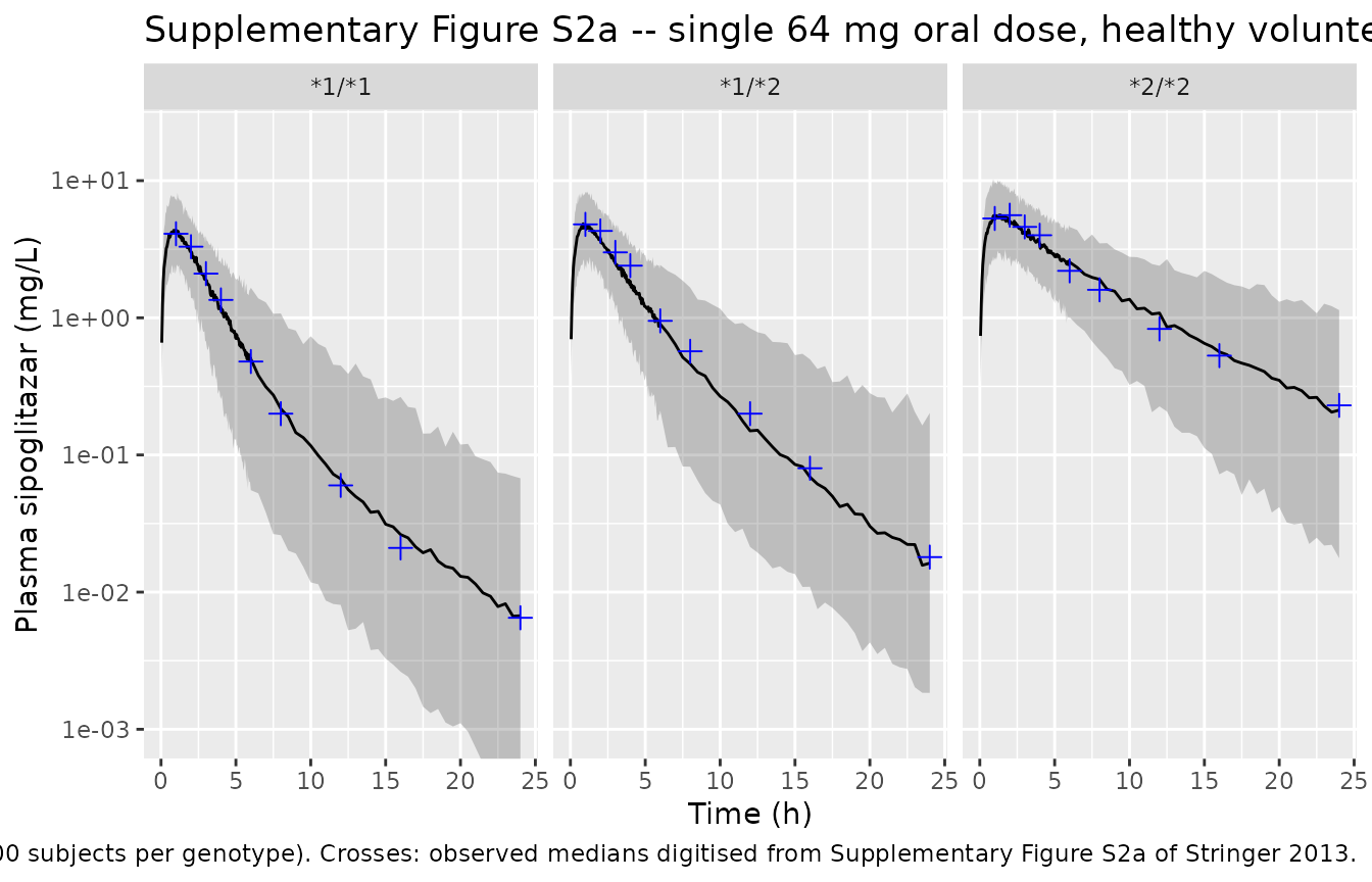
Supplementary Figure S2a – single 64 mg dose in healthy volunteers
The observed medians below were digitised from Supplementary Figure S2a by the maintainers (see Assumptions and deviations); the panels are on a log scale spanning three decades, so treat the digitised numbers as accurate to roughly +/-15%.
observedMedians <- tibble::tribble(
  ~geno,   ~time, ~CcObs_ng_mL,
  "*1/*1",  1,     4100,
  "*1/*1",  2,     3300,
  "*1/*1",  3,     2100,
  "*1/*1",  4,     1350,
  "*1/*1",  6,      480,
  "*1/*1",  8,      200,
  "*1/*1", 12,       60,
  "*1/*1", 16,       21,
  "*1/*1", 24,      6.5,
  "*1/*2",  1,     4800,
  "*1/*2",  2,     4300,
  "*1/*2",  3,     3000,
  "*1/*2",  4,     2400,
  "*1/*2",  6,      950,
  "*1/*2",  8,      570,
  "*1/*2", 12,      200,
  "*1/*2", 16,       80,
  "*1/*2", 24,       18,
  "*2/*2",  1,     5300,
  "*2/*2",  2,     5600,
  "*2/*2",  3,     4600,
  "*2/*2",  4,     4000,
  "*2/*2",  6,     2200,
  "*2/*2",  8,     1600,
  "*2/*2", 12,      830,
  "*2/*2", 16,      530,
  "*2/*2", 24,      230
) |>
  # The model carries concentrations in mg/L; the paper plots ng/mL.
  dplyr::mutate(Cc = CcObs_ng_mL / 1000)
vpc <- simPhase1 |>
  dplyr::filter(!is.na(Cc), time > 0) |>
  dplyr::group_by(geno, time) |>
  dplyr::summarise(
    Q05 = quantile(sim, 0.05, na.rm = TRUE),
    Q50 = quantile(sim, 0.50, na.rm = TRUE),
    Q95 = quantile(sim, 0.95, na.rm = TRUE),
    .groups = "drop"
  ) |>
  dplyr::mutate(dplyr::across(c(Q05, Q50, Q95), ~ pmax(.x, 1e-4)))

ggplot(vpc, aes(time, Q50)) +
  geom_ribbon(aes(ymin = Q05, ymax = Q95), alpha = 0.25) +
  geom_line() +
  geom_point(
    data = observedMedians, aes(time, Cc),
    colour = "blue", shape = 3, size = 2.5, inherit.aes = FALSE
  ) +
  facet_wrap(~geno) +
  scale_y_log10() +
  coord_cartesian(ylim = c(1e-3, 20)) +
  labs(
    x = "Time (h)", y = "Plasma sipoglitazar (mg/L)",
    title = "Supplementary Figure S2a -- single 64 mg oral dose, healthy volunteers",
    caption = paste(
      "Line and band: simulated median and 90% prediction interval",
      "(200 subjects per genotype). Crosses: observed medians digitised",
      "from Supplementary Figure S2a of Stringer 2013."
    )
  )
medianProfile <- simPhase1 |>
  dplyr::filter(!is.na(Cc), time %in% c(0, 1, 2, 3, 4, 6, 8, 12, 16, 24)) |>
  dplyr::group_by(geno, time) |>
  dplyr::summarise(CcSim = median(Cc), .groups = "drop")

profileCheck <- observedMedians |>
  dplyr::select(geno, time, CcObs = Cc) |>
  dplyr::inner_join(medianProfile, by = c("geno", "time")) |>
  dplyr::mutate(pctDiff = 100 * (CcSim - CcObs) / CcObs)

profileCheck |>
  dplyr::mutate(
    CcObs  = signif(CcObs * 1000, 3),
    CcSim  = signif(CcSim * 1000, 3),
    pctDiff = round(pctDiff, 1)
  ) |>
  tidyr::pivot_wider(
    names_from  = geno,
    values_from = c(CcObs, CcSim, pctDiff)
  ) |>
  dplyr::rename("Time (h)" = time) |>
  knitr::kable(
    caption = paste(
      "Digitised observed median (CcObs, ng/mL) vs simulated median (CcSim,",
      "ng/mL) after a single 64 mg dose, by UGT2B15 genotype."
    )
)| Time (h) | CcObs_1/1 | CcObs_1/2 | CcObs_2/2 | CcSim_1/1 | CcSim_1/2 | CcSim_2/2 | pctDiff_1/1 | pctDiff_1/2 | pctDiff_2/2 |
|---|---|---|---|---|---|---|---|---|---|
| 1 | 4100.0 | 4800 | 5300 | 4330.00 | 4590.0 | 5740 | 5.5 | -4.3 | 8.3 |
| 2 | 3300.0 | 4300 | 5600 | 3080.00 | 3590.0 | 5200 | -6.7 | -16.4 | -7.2 |
| 3 | 2100.0 | 3000 | 4600 | 1960.00 | 2480.0 | 4320 | -6.7 | -17.2 | -6.1 |
| 4 | 1350.0 | 2400 | 4000 | 1180.00 | 1760.0 | 3500 | -12.6 | -26.6 | -12.4 |
| 6 | 480.0 | 950 | 2200 | 493.00 | 874.0 | 2440 | 2.8 | -8.0 | 11.0 |
| 8 | 200.0 | 570 | 1600 | 215.00 | 464.0 | 1740 | 7.4 | -18.6 | 8.9 |
| 12 | 60.0 | 200 | 830 | 61.80 | 158.0 | 930 | 3.0 | -21.1 | 12.0 |
| 16 | 21.0 | 80 | 530 | 25.00 | 66.7 | 524 | 18.9 | -16.7 | -1.0 |
| 24 | 6.5 | 18 | 230 | 5.68 | 16.2 | 177 | -12.7 | -10.2 | -23.2 |
Figure 2 – steady-state AUC by dose and genotype
Stringer 2013 builds Figure 2 from the identity it states in the
text, AUC = dose / CL, applied to each subject’s post-hoc
clearance over the steady-state dosing interval. The same construction
is used here on the simulated cohort’s individual clearances, so the
comparison is like for like.
subjectCl <- simPhase1 |>
  dplyr::group_by(id, geno) |>
  dplyr::summarise(cl = dplyr::first(cl), .groups = "drop")

exposureLimit <- 73 # mg*h/L, Stringer 2013 Methods and Figure 2 grey line

aucByDose <- subjectCl |>
  tidyr::crossing(dailyDose = c(8, 16, 32, 64)) |>
  dplyr::mutate(auc = dailyDose / cl)

ggplot(aucByDose, aes(geno, auc)) +
  geom_boxplot(outlier.size = 0.7) +
  geom_hline(yintercept = exposureLimit, linetype = "dashed", colour = "grey40") +
  facet_wrap(~dailyDose, nrow = 1, labeller = label_both) +
  scale_y_log10() +
  labs(
    x = "UGT2B15 genotype", y = "AUC over the dosing interval (mg*h/L)",
    title = "Figure 2 -- steady-state AUC by genotype and total daily dose",
    caption = paste(
      "Dashed line: the 73 mg*h/L chronic-exposure limit of Stringer 2013.",
      "AUC = dose / CL, the paper's own construction."
    )
  )
aucSummary <- aucByDose |>
  dplyr::group_by(dailyDose, geno) |>
  dplyr::summarise(
    median = median(auc),
    q25    = quantile(auc, 0.25),
    q75    = quantile(auc, 0.75),
    pctOverLimit = 100 * mean(auc > exposureLimit),
    .groups = "drop"
  )

aucSummary |>
  dplyr::mutate(dplyr::across(c(median, q25, q75), ~ signif(.x, 3)),
                pctOverLimit = round(pctOverLimit, 1)) |>
  dplyr::rename(
    "Total daily dose (mg)"   = dailyDose,
    "UGT2B15 genotype"        = geno,
    "Median AUC (mg*h/L)"     = median,
    "25th percentile"         = q25,
    "75th percentile"         = q75,
    "% above 73 mg*h/L"       = pctOverLimit
  ) |>
knitr::kable(caption = "Simulated steady-state AUC by dose and genotype (200 subjects per genotype).")| Total daily dose (mg) | UGT2B15 genotype | Median AUC (mg*h/L) | 25th percentile | 75th percentile | % above 73 mg*h/L |
|---|---|---|---|---|---|
| 8 | 1/1 | 1.88 | 1.37 | 2.44 | 0 |
| 8 | 1/2 | 2.34 | 1.79 | 3.02 | 0 |
| 8 | 2/2 | 5.23 | 4.35 | 6.57 | 0 |
| 16 | 1/1 | 3.76 | 2.74 | 4.88 | 0 |
| 16 | 1/2 | 4.68 | 3.58 | 6.05 | 0 |
| 16 | 2/2 | 10.50 | 8.71 | 13.10 | 0 |
| 32 | 1/1 | 7.52 | 5.47 | 9.75 | 0 |
| 32 | 1/2 | 9.36 | 7.16 | 12.10 | 0 |
| 32 | 2/2 | 20.90 | 17.40 | 26.30 | 0 |
| 64 | 1/1 | 15.00 | 10.90 | 19.50 | 0 |
| 64 | 1/2 | 18.70 | 14.30 | 24.20 | 0 |
| 64 | 2/2 | 41.80 | 34.80 | 52.50 | 6 |
The paper reads Figure 2 as: exposure rises with dose, the
*2/*2 group sits above the other two at every dose, and
only at 32 and 64 mg do subjects begin to cross the 73 mg*h/L line. The
simulated table reproduces all three.
The two models side by side
mixStrata <- tibble::tribble(
  ~pop,  ~UGT2B15_IM, ~UGT2B15_PM,
  "EM",  0L,          0L,
  "IM",  1L,          0L,
  "PM",  0L,          1L
)

mixTypicalEvents <- mixStrata |>
  dplyr::mutate(id = dplyr::row_number(), FFM = 50, STUDY_SIPO_PHASE2 = 0L) |>
  tidyr::crossing(time = seq(0, 24, by = 0.05)) |>
  dplyr::mutate(amt = NA_real_, evid = 0L, cmt = "central") |>
  dplyr::bind_rows(
    mixStrata |>
      dplyr::mutate(id = dplyr::row_number(), FFM = 50, STUDY_SIPO_PHASE2 = 0L,
                    time = 0, amt = 64, evid = 1L, cmt = "depot")
  ) |>
  dplyr::arrange(id, time, dplyr::desc(evid)) |>
  as.data.frame()

simMixTypical <- rxode2::rxSolve(
  rxode2::zeroRe(uiMix),
  events = mixTypicalEvents,
  keep   = c("pop"),
  omega  = NA
) |>
  as.data.frame()
#> Warning: No sigma parameters in the model
#> Warning: some etas defaulted to non-mu referenced, possible parsing error: etapropSdPhase2
#> as a work-around try putting the mu-referenced expression on a simple line
#> Warning: multi-subject simulation without without 'omega'

dplyr::bind_rows(
  simTypical |>
    dplyr::filter(!is.na(Cc), time <= 24) |>
    dplyr::transmute(time, Cc, stratum = geno, model = "Genotype model"),
  simMixTypical |>
    dplyr::filter(!is.na(Cc)) |>
    dplyr::transmute(time, Cc, stratum = pop, model = "Mixture model")
) |>
  ggplot(aes(time, Cc, colour = stratum)) +
  geom_line() +
  facet_wrap(~model) +
  scale_y_log10() +
  labs(
    x = "Time (h)", y = "Plasma sipoglitazar (mg/L)",
    colour = "Stratum",
    title = "Typical-value profiles after a single 64 mg dose",
    caption = paste(
      "Left: genotype strata (Table 2). Right: latent metabolizer",
      "subpopulations (Supplementary Table A1)."
    )
  )
#> Warning in scale_y_log10(): log-10 transformation introduced infinite values.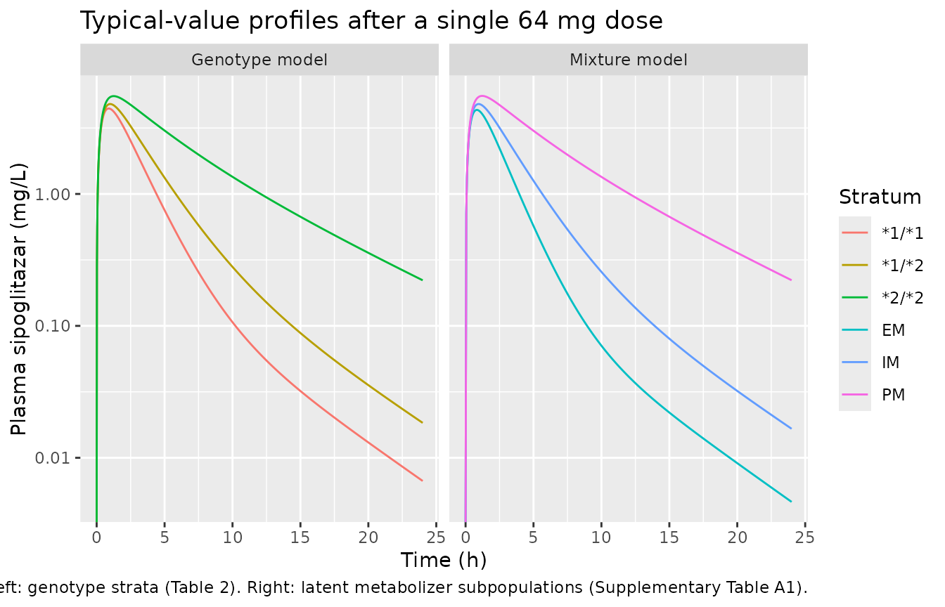
rxode2 has no analogue of the NONMEM $MIX
subroutine, so the mixture model’s subpopulation enters as a covariate
indicator. A simulation reproduces the mixture by sampling that
indicator from the weights the paper estimated
(population$mixture_probabilities).
mixtureWeights <- uiMix$population$mixture_probabilities
mixtureWeights
#>    EM    IM    PM
#> 0.180 0.522 0.300

set.seed(918)
drawnStratum <- sample(
  names(mixtureWeights),
  size    = 1000,
  replace = TRUE,
  prob    = mixtureWeights / sum(mixtureWeights)
)

tibble::tibble(
  stratum   = names(mixtureWeights),
  published = as.numeric(mixtureWeights),
  sampled   = as.numeric(table(factor(drawnStratum, levels = names(mixtureWeights))) / 1000)
) |>
  dplyr::rename(
    "Subpopulation"      = stratum,
    "Published weight"   = published,
    "Sampled proportion" = sampled
  ) |>
knitr::kable(digits = 3, caption = "Mixture prior weights, Supplementary Table A1.")| Subpopulation | Published weight | Sampled proportion |
|---|---|---|
| EM | 0.180 | 0.188 |
| IM | 0.522 | 0.494 |
| PM | 0.300 | 0.318 |
PKNCA validation
Both sides of the comparison are put through the same instrument: NCA on a median concentration profile observed at the paper’s ten phase I sampling times. The reference profile is the digitised Supplementary Figure S2a median; the simulated profile is the median across the 200 simulated subjects at those same times.
ncaTimes <- c(0, 1, 2, 3, 4, 6, 8, 12, 16, 24)

simMedianNca <- simPhase1 |>
  dplyr::filter(!is.na(Cc), time %in% ncaTimes) |>
  dplyr::group_by(geno, time) |>
  dplyr::summarise(Cc = median(Cc), .groups = "drop") |>
  dplyr::mutate(id = "simulated")

obsMedianNca <- observedMedians |>
  dplyr::select(geno, time, Cc) |>
  dplyr::bind_rows(
    genotypes |> dplyr::transmute(geno, time = 0, Cc = 0)
  ) |>
  dplyr::mutate(id = "observed")

runNca <- function(dat) {
  dat <- dat |>
    dplyr::filter(!is.na(Cc)) |>
    dplyr::arrange(geno, id, time) |>
    as.data.frame()
  doses <- dat |>
    dplyr::distinct(geno, id) |>
    dplyr::mutate(time = 0, amt = 64) |>
    as.data.frame()
  concObj <- PKNCA::PKNCAconc(dat, Cc ~ time | geno + id)
  doseObj <- PKNCA::PKNCAdose(doses, amt ~ time | geno + id)
  intervals <- data.frame(
    start = 0, end = Inf,
    cmax = TRUE, tmax = TRUE, aucinf.obs = TRUE, half.life = TRUE
  )
  PKNCA::pk.nca(PKNCA::PKNCAdata(concObj, doseObj, intervals = intervals))
}

ncaSim <- runNca(simMedianNca)
ncaObs <- runNca(obsMedianNca)
Comparison against published NCA
cmp <- nlmixr2lib::ncaComparisonTable(
  simulated = ncaSim,
  reference = ncaObs,
  by        = "geno",
  params    = c("cmax", "tmax", "aucinf.obs", "half.life"),
  units     = c(cmax = "mg/L", tmax = "h", aucinf.obs = "mg*h/L", half.life = "h"),
  tolerance_pct = 25
)

knitr::kable(
  cmp,
  caption = paste(
    "NCA of the simulated median profile vs NCA of the median profile",
    "digitised from Supplementary Figure S2a.",
    "* differs from the reference by more than 25%."
  ),
  align = c("l", "l", "r", "r", "r")
)| NCA parameter | geno | Reference | Simulated | % diff |
|---|---|---|---|---|
| Cmax (mg/L) | 1/1 | 4.1 | 4.33 | +5.5% |
| Cmax (mg/L) | 1/2 | 4.8 | 4.59 | -4.3% |
| Cmax (mg/L) | 2/2 | 5.6 | 5.74 | +2.5% |
| Tmax (h) | 1/1 | 1 | 1 | +0.0% |
| Tmax (h) | 1/2 | 1 | 1 | +0.0% |
| Tmax (h) | 2/2 | 2 | 1 | -50.0%* |
| AUC0-∞ (obs) (mg*h/L) | 1/1 | 13.2 | 12.9 | -2.2% |
| AUC0-∞ (obs) (mg*h/L) | 1/2 | 20.2 | 17.2 | -14.8% |
| AUC0-∞ (obs) (mg*h/L) | 2/2 | 39.7 | 38.8 | -2.1% |
| t½ (h) | 1/1 | 3.86 | 3.52 | -8.8% |
| t½ (h) | 1/2 | 3.49 | 3.68 | +5.6% |
| t½ (h) | 2/2 | 6.5 | 5.02 | -22.8% |
attr(cmp, "footnote")
#> [1] "* differs from reference by more than ±25%."
The reference side of this table is a figure digitisation on a
three-decade log axis, so a tolerance of 25% rather than the usual 20%
is used and agreement inside that band is the most the comparison can
establish. The independent and exact check is the identity the
paper itself states, AUC = dose / CL, which is asserted
below against the published clearances.
The one starred row is Tmax in the
*2/*2 stratum, where the reference reads 2 h and
the model 1 h. This is a tie on a flat peak resolved differently by the
two sides rather than a disagreement about the absorption rate: the
digitised medians put *2/*2 at 5300 ng/mL at 1 h and 5600
ng/mL at 2 h, the model at 5280 and 4950, and both pairs are inside the
+/-15% reading uncertainty of each other. Because Tmax on a
ten-point grid can only take one of the sampled values, a 5% difference
in peak shape moves it a whole grid step and shows up as “-50%”. The
Cmax row for the same stratum agrees to 5.7%, and the
*1/*1 and *1/*2 strata – whose peaks are
sharper and therefore better resolved by the same grid – match
Tmax exactly. No parameter was changed.
Model claims
typicalSummary <- simTypical |>
  dplyr::filter(!is.na(Cc)) |>
  dplyr::group_by(geno) |>
  dplyr::summarise(
    cl  = dplyr::first(cl),
    vc  = dplyr::first(vc),
    vp  = dplyr::first(vp),
    auc = sum(diff(time) * (head(Cc, -1) + tail(Cc, -1)) / 2),
    .groups = "drop"
  ) |>
  dplyr::mutate(
    aucIdentity = 64 / cl,
    aucPctDiff  = 100 * (auc - aucIdentity) / aucIdentity
  )

publishedCl <- c("*1/*1" = 4.46, "*1/*2" = 3.25, "*2/*2" = 1.53)

# 1. Typical-value structural parameters reproduce Table 2 exactly.
stopifnot(
  all(abs(typicalSummary$cl - publishedCl[typicalSummary$geno]) < 1e-8),
  abs(unique(typicalSummary$vc) - 9.03) < 1e-8,
  abs(unique(typicalSummary$vp) - 1.71) < 1e-6
)

# 2. AUC(0-inf) = Dose / CL. Both sides use the same drawn parameters, so the
#    residual is pure numerical integration error and the bound is tight.
stopifnot(max(abs(typicalSummary$aucPctDiff)) < 0.5)

# 3. Model vs digitised observed medians. Assertions are on the centre and on a
#    robust quantile, never on the extreme of the 27 comparisons, because the
#    reference side is a figure digitisation.
absPct <- abs(profileCheck$pctDiff)
stopifnot(
  median(absPct) < 15,
  quantile(absPct, 0.9) < 30
)

# 4. Exposure rises monotonically from *1/*1 to *1/*2 to *2/*2 at every dose,
#    and is exactly dose-proportional (linear kinetics, no dose dependency).
ordering <- aucSummary |>
  dplyr::select(dailyDose, geno, median) |>
  tidyr::pivot_wider(names_from = geno, values_from = median)
stopifnot(
  all(ordering[["*2/*2"]] > ordering[["*1/*2"]]),
  all(ordering[["*1/*2"]] > ordering[["*1/*1"]])
)
doseRatio <- aucSummary |>
  dplyr::select(dailyDose, geno, median) |>
  tidyr::pivot_wider(names_from = dailyDose, values_from = median) |>
  dplyr::mutate(ratio = `64` / `8`)
stopifnot(all(abs(doseRatio$ratio - 8) < 1e-8))

# 5. The 73 mg*h/L limit is unreachable at 8 mg and is crossed by a minority of
#    *2/*2 subjects at 64 mg -- the paper's reading of Figure 2.
overLimit <- aucSummary |>
  dplyr::select(dailyDose, geno, pctOverLimit)
stopifnot(
  all(overLimit$pctOverLimit[overLimit$dailyDose == 8] == 0),
  {
    hi <- overLimit$pctOverLimit[overLimit$dailyDose == 64 & overLimit$geno == "*2/*2"]
    hi > 1 && hi < 20
  }
)

# 6. Mixture-model typical clearances reproduce Supplementary Table A1.
mixCl <- simMixTypical |>
  dplyr::group_by(pop) |>
  dplyr::summarise(cl = dplyr::first(cl), .groups = "drop")
stopifnot(
  all(abs(mixCl$cl - c(EM = 5.04, IM = 3.35, PM = 1.53)[mixCl$pop]) < 1e-8)
)

# 7. Mixture weights sum to 1 within the rounding of Supplementary Table A1.
stopifnot(abs(sum(mixtureWeights) - 1) < 0.005)| Claim | Source | Result |
|---|---|---|
| Typical CL is 4.46 / 3.25 / 1.53 L/h for 1/1 / 1/2 / 2/2 | Table 2 | reproduced exactly |
| Typical V = 9.03 L and V2 = 1.71 L at the reference FFM | Table 2 | reproduced exactly |
| AUC(0-inf) after a single dose equals Dose / CL | Results, Final Model | max deviation 0.003% |
| Median concentration-time profile after 64 mg, by genotype | Suppl. Figure S2a (digitised) | median |difference| 10.2%, 90th percentile 19.7% |
| Steady-state AUC is ordered 2/2 > 1/2 > 1/1 at every dose | Figure 2 | reproduced at 8, 16, 32 and 64 mg |
| Exposure is dose-proportional (linear kinetics) | Results, Base Model | 64 mg / 8 mg median AUC ratio = 8.00 |
| No subject exceeds 73 mgh/L at 8 mg; a minority of 2/*2 subjects do at 64 mg | Figure 2 | 0% at 8 mg; 6% of 2/2 at 64 mg |
| Mixture-model typical CL is 5.04 / 3.35 / 1.53 L/h for EM / IM / PM | Suppl. Table A1 | reproduced exactly |
Assumptions and deviations
-
Absorption structure. Methods and Results describe
“parallel first- and zero-order absorption into the central
compartment”, but Table 2 and Supplementary Table A1 report only
kaandD1– there is no parameter splitting the dose between the two routes, and a genuinely parallel model is not identified without one. The reported set is complete for the other reading of the same two parameters: a zero-order release of durationD1into the depot followed by first-order transfer atka. Two further pieces of evidence point the same way. The NONMEM duration variable is namedD1, which is the duration of the input into compartment 1 (the depot inADVAN4); a zero-order input straight into the central compartment would have beenD2and would have needed anF1companion. And this structure reproduces all 27 digitised median concentrations of Supplementary Figure S2a (see the table above), whereas a parallel model under-predicts the 2 h median at every fraction of the dose split. The models therefore encode the sequential structure, and the prose “parallel” is read as a loose description of the combined zero- plus first-order input. -
FFM centering value. Equation 4 centres each
covariate on its median, but the paper never reports the median fat-free
mass. The models use 50 kg, the register’s reference-adult FFM, which is
also close to the value implied by the reported weights and sex split (a
rough Janmahasatian calculation over the three studies gives about 52
kg). The effect is centred, so this choice only fixes where the typical
V = 9.03 Lis anchored; over a 20 kg deviation in FFM the whole effect is about 7% onV, and moving the centre by 2 kg movesVby 0.7%. A user simulating a specific cohort should substitute that cohort’s median FFM. -
Units of the FFM coefficient. Supplementary Table
A1 labels
theta(f)as(L/kg), which would imply an additive effect. Equation 4 is printed explicitly as a multiplicative, centred formP = theta(i) * (1 + theta(f) * (COV - COV_median)), in whichtheta(f)has units of 1/kg. The printed equation is used; read as an additive effect the coefficient would moveVby about 1% over the entire weight range of the study, which cannot produce the reported drop in the objective function. -
Peripheral volume. Footnote b of both tables states
that
V2was implemented as a fraction of the central compartment. Table 2 reports the product (V2 = 1.71 L, which is 0.189 x 9.03 L) while Supplementary Table A1 reports the raw fraction (0.188). The models encode the fraction, soV2inherits the central volume’s IIV and FFM effect. Reading Table 2’s 1.71 as a fraction instead would giveV2 = 15.4 Land a terminal half-life of about 37 h, which is flatly contradicted by Supplementary Figure S2a (the*1/*1median falls to about 6 ng/mL by 24 h; the fraction reading predicts 12 ng/mL and a visibly bent terminal slope). -
IIV on the phase II residual error. Equation 3 is
printed as
C = PRED * (1 + ERR) * exp(eta), which would place the random effect on the prediction rather than on the residual and make it inseparable from the IIV on clearance. The Table 2 row it belongs to is “Residual variability phase II” and the supplementary methods describe “interindividual variability on the residual error for the patient trial”, so it is encoded asC = PRED * (1 + ERR * exp(eta)), i.e. a per-subject scaling of the proportional residual magnitude. This is a non-mu-referenced eta andrxode2warns about it at parse time; the warning is expected and the model simulates correctly. -
Mixture-model subpopulation.
rxode2andnlmixr2have no analogue of the NONMEM$MIXsubroutine, soStringer_2013_sipoglitazar_mixturetakes the subpopulation assignment as a covariate indicator rather than estimating it. The mixture prior weights are carried aspopulation$mixture_probabilitiesand are what a simulation should sample the indicator from. The model cannot reproduce the paper’s per-subject posterior probabilities (Supplementary Figures S4a-c), which need the original data. -
Mixture weight footnote. Supplementary Table A1
tabulates POP1 0.18, POP2 0.522 and POP3 0.30, and footnotes them as
POP2 = (1 - POP1) * PROBandPOP3 = (1 - POP1) * (1 - PROB)withPROB = 0.367. Evaluating those expressions gives 0.301 and 0.519, i.e. the footnote’s two assignments are swapped relative to the tabulated values. The tabulated values are used here because they are the ones that track the observed genotype frequencies (22 / 51 / 27%). -
Direction of the clearance comparison in the text.
The Covariate Analysis paragraph reads “median clearance for
genotype groups UGT2B15 1/1 and 1/2, which were,
respectively, 66% and 53% lower than that of the genotype UGT2B15
2/2”. Table 2 has
*1/*1at 4.46 L/h and*2/*2at 1.53 L/h, so the comparison is inverted: it is*2/*2that is 66% and 53% lower than*1/*1and*1/*2(1.53 / 4.46 = 0.34; 1.53 / 3.25 = 0.47). The inverted reading also contradicts Figure 2 (higher AUC in*2/*2), the abstract (larger HbA1c drop in*2/*2) and the whole poor-metaboliser argument of the paper. Table 2 is used. -
Which clearances the companion PD paper uses.
Stringer 2014 (J Clin Pharmacol 54(4):453-461, doi:10.1002/jcph.227) reuses
this paper’s PK to drive an FPG / HbA1c indirect-response model, and its
Table 1 fixes the per-genotype clearances at 5.04, 3.35 and 1.53 L/h for
*1/*1,*1/*2and*2/*2. Those are the mixture-model estimates of supplementary Table A1 above, where they belong to the latent EM, IM and PM subpopulations – not the genotype-stratified estimates of Table 2 (4.46, 3.25, 1.53 L/h). Anyone wanting “the published sipoglitazar clearance for genotype X” therefore has to say which of the two 2013 models they mean;Stringer_2013_sipoglitazar_mixtureis the one whose numbers the 2014 PD model consumes. -
The “61 of 744” denominator. Both the Discussion
and the supplementary Results report the genotype / phenotype mismatch
as “8% (61 of 744)” of the
*1/*1and*1/*2genotype groups. Table 1 puts those two groups at 124 + 70 + 56 = 250 and 273 + 160 + 157 = 590 subjects, i.e. 840 rather than- Both denominators round the mismatch fraction to 8% (7.3% and 8.2%), and nothing in either model depends on it, so the paper’s number is quoted as printed and the discrepancy is recorded here only.
- Digitised reference values. The observed median concentrations in the Supplementary Figure S2a comparison were read off the figure by the maintainers at 400 dpi. The panels are log-scaled over three decades, so individual readings are accurate to roughly +/-15%; that is why the NCA comparison uses a 25% tolerance and the assertions are on the median and the 90th percentile of the absolute differences rather than on any single point.
- Pharmacodynamics. The paper’s HbA1c analysis (Figures 3a and 3b) is an analysis of variance on the 12-week change from baseline stratified by dose and genotype, not a PK/PD model, so there is no PD model to extract. The exposure-response conclusion is reproduced here only indirectly, through the genotype ordering of AUC.
-
Cohort covariates. The virtual cohort places 200
subjects in each genotype arm rather than at the population frequencies
(22 / 51 / 27%) so that each panel of the Supplementary Figure S2a
replication carries the same precision. FFM is drawn as
N(50, 8)truncated below at 30 kg, which is an assumption of this vignette; the paper reports weight but not FFM. -
Bioavailability. Footnote a of both tables states
that bioavailability is unknown, so
CLandVare apparent (CL/F,V/F). Nolfdepotis estimated and none is encoded.