Colistin / CMS (Mohamed 2012)
Source:vignettes/articles/Mohamed_2012_colistin.Rmd
Mohamed_2012_colistin.RmdModel and source
- Citation: Mohamed AF, Karaiskos I, Plachouras D, Karvanen M, Pontikis K, Jansson B, Papadomichelakis E, Antoniadou A, Giamarellou H, Armaganidis A, Cars O, Friberg LE. “Application of a Loading Dose of Colistin Methanesulfonate in Critically Ill Patients: Population Pharmacokinetics, Protein Binding, and Prediction of Bacterial Kill.” Antimicrobial Agents and Chemotherapy 2012; 56(8):4241-4249.
- DOI: https://doi.org/10.1128/AAC.06426-11
- Upstream popPK structure shared with: Plachouras et al. 2009 Antimicrob Agents Chemother 53:3430-3436 (reference 34 in the source).
- Upstream semimechanistic PKPD source: Mohamed AF, Cars O, Friberg LE. 2011. PAGE meeting abstract 2223 (reference 29 in the source).
Population
The model was fit to the combined N = 28 critically ill cohort consisting of:
- n = 10 patients enrolled prospectively at the Attikon University Hospital Critical Care Unit (Athens) between July 2009 and January 2010, receiving a 480 mg (6 MU) CMS loading dose followed by maintenance dosing of 80-240 mg (1-3 MU) every 8 h or 30-90 mg every 12 h (15-minute IV infusions). Baseline demographics are tabulated in Mohamed 2012 Table 1: 6 males / 4 females, ages 32-88 years (mean 55.4), body weight 60-140 kg, APACHE II scores 7-23, serum creatinine 0.6-1.7 mg/dL, baseline CrCL 24.9-214.3 mL/min, serum albumin 1.9-3.8 g/dL. Most patients had ventilator-associated pneumonia; one had bacteremia and one acute mesenteric ischemia. Patients on continuous venovenous hemodiafiltration were excluded.
- n = 18 patients from Plachouras et al. 2009 (reference 34), who received the older 240 mg (3 MU) q8h regimen without a loading dose. Samples were pooled for simultaneous PK analysis (267 CMS / colistin concentration measurements total).
The same information is available programmatically via
readModelDb("Mohamed_2012_colistin")$population.
Source trace
Per-parameter origin is recorded as in-file comments next to each
ini() entry in
inst/modeldb/specificDrugs/Mohamed_2012_colistin.R. The
table below collects them in one place for review.
| Element | Value / form | Source location |
|---|---|---|
| CL_CMS | 13.1 L/h | Table 2 (“Typical value” column, CMS row “CL_CMS or CL_col”) |
| V1_CMS | 11.8 L | Table 2 (CMS row “V1 or V_col”) |
| Q_CMS | 206 L/h | Table 2 (CMS row “Q”) |
| V2_CMS | 28.4 L | Table 2 (CMS row “V2”) |
| Apparent CL_col / f_m | 8.2 L/h | Table 2 (Colistin row “CL_CMS or CL_col”); f_m is the unknown fraction of CMS metabolized to colistin (Materials and Methods, “Population pharmacokinetic modeling”) |
| Apparent V_col / f_m | 218 L | Table 2 (Colistin row “V1 or V_col”) |
| IIV(CL_CMS) = 42 % | etalcl variance | Table 2 (CMS row, IIV column 42 % with 90% CI 21-42.3) |
| IIV(Q_CMS) = 111 % | etalq variance | Table 2 (CMS row Q, IIV 111 % with 90% CI 52-197) |
| IIV(CL_col) = 76 % = 1.8 x IIV(CL_CMS) | 1.8 x etalcl | Table 2 (Colistin row, IIV 76 % with footnote: “value obtained when the variability of CL_col was scaled from the variability of CL_CMS by the estimated value of 1.8 (90% CI 1.4-2.9)”). 100% correlation reported (paper Results “PK model”: “Inclusion of covariance between CL_CMS and CL_col improved the OFV further [27 units], and as the correlation was estimated to be 100% …”). |
| IOV(CL_CMS) = 30 % | implemented as added eta on log scale | Table 2 IOV column |
| IOV(V2_CMS) = 59 % | etalvp | Table 2 IOV column |
| IOV(CL_col) = 48 % | etalcl_col | Table 2 IOV column |
| IOV(V_col) = 48 % | etalvc_col | Table 2 IOV column |
| CMS proportional residual SD | 0.23 | Table 2 (CMS row, “Proportional error (%)” 0.23 with 90% CI 0.12-0.21) |
| CMS additive residual SD | 0.071 umol/L | Table 2 (CMS row, “Additive residual error (umol/L)”) |
| Colistin proportional residual SD | 0.082 | Table 2 (Colistin row) |
| Colistin additive residual SD | 0.044 umol/L | Table 2 (Colistin row) |
| CMS molar mass 1743 g/mol | unit conversion | Materials and Methods, “Analytical method” |
| Colistin molar mass 1163 g/mol | unit conversion | Materials and Methods, “Analytical method” |
| f_uA = 31.2 x CA / (0.094 + CA) | Eq 3 | Results, “Plasma protein binding”; Eq 3 |
| f_uB = 0.43 | constant | Results, “Plasma protein binding”: “f_uB … was found to be constant (average, 43 %)” |
| CA / CB = 3.6 (mean) | constant | Results “CMS and colistin concentrations”: “ratio … ranged from 2.5 to 4.8 … appeared to be constant within and between dosing intervals over an individual time”; “average ratio of CA to CB (3.6)” in “Predictions of bacterial kill” |
| Emax (max kill rate) = 35 1/h | Materials and Methods, “Predictions of bacterial kill” | |
| EC50 = 2.9 mg/L (unbound colistin) | Materials and Methods, “Predictions of bacterial kill” | |
| Bacterial growth rate = 0.99 1/h | Materials and Methods, “Predictions of bacterial kill” | |
| Bacterial natural death = 0.18 1/h | Materials and Methods, “Predictions of bacterial kill” | |
| Emergence of resistance = 6.0e-5 L/(mg*h) | rate constant | Materials and Methods, “Predictions of bacterial kill” |
| Reversal of resistance = 0.15 1/h | Materials and Methods, “Predictions of bacterial kill” | |
| Maximum bacterial count = 1.8e8 CFU/mL | Materials and Methods, “Predictions of bacterial kill” | |
| Initial inoculum = 4.5e5 CFU/mL | Materials and Methods, “Predictions of bacterial kill” |
The CMS to colistin formation flux is encoded as
cl * (central_cms / vc) (the full CMS clearance times CMS
concentration). The apparent-amount parametrisation of the colistin
compartment absorbs the unknown f_m factor: the colistin compartment
“amount” represents A_real / f_m, and the observed colistin
concentration recovered as A_apparent / V_col_apparent is
the actual (real) plasma colistin concentration the paper modelled.
Virtual cohort
set.seed(2012L)
n_subj <- 50L
cohort <- tibble::tibble(
  id  = seq_len(n_subj),
  WT  = round(stats::runif(n_subj, 60, 140), 1),  # Table 1 actual body weight range
  AGE = round(stats::runif(n_subj, 32, 88))       # Table 1 age range
)
head(cohort)
#> # A tibble: 6 × 3
#>      id    WT   AGE
#>   <int> <dbl> <dbl>
#> 1     1  77.5    65
#> 2     2 120.     74
#> 3     3  82.5    87
#> 4     4 135.     52
#> 5     5 120.     78
#> 6     6 130      71
The covariate columns are carried in the dataset for downstream NCA-by-strata analyses, but the final model has no covariate effects (see Errata).
Simulation
The same simulation is reused for the published-figure replications and the PKNCA validation table.
mod <- readModelDb("Mohamed_2012_colistin")

cms_dose_mg_per_15min <- function(amt_mg) amt_mg / (15 / 60)  # rate (mg/h) for a 15-min infusion

# Loading-dose regimen: 480 mg load then 240 mg q8h for 32 hours
build_events <- function(cohort) {
  doses <- lapply(seq_len(nrow(cohort)), function(i) {
    id <- cohort$id[i]
    dplyr::bind_rows(
      tibble::tibble(id = id, time = 0,  amt = 480, rate = cms_dose_mg_per_15min(480),
                     cmt = "central_cms", evid = 1L),
      tibble::tibble(id = id, time = 8,  amt = 240, rate = cms_dose_mg_per_15min(240),
                     cmt = "central_cms", evid = 1L),
      tibble::tibble(id = id, time = 16, amt = 240, rate = cms_dose_mg_per_15min(240),
                     cmt = "central_cms", evid = 1L),
      tibble::tibble(id = id, time = 24, amt = 240, rate = cms_dose_mg_per_15min(240),
                     cmt = "central_cms", evid = 1L)
    )
  })
  obs_times <- seq(0.05, 32, length.out = 200)
  # One observation row per (id, time). rxode2 evaluates every output column
  # (Ccms, Cc_col, logCFU) on every observation row regardless of the cmt
  # tag; the cmt tag only routes residual error to the matching output. Using
  # `cmt = "Ccms"` here keeps PKNCA happy (no duplicate (id, time) rows) and
  # still gives us Cc_col / logCFU columns to plot.
  obs <- do.call(rbind, lapply(cohort$id, function(id) {
    tibble::tibble(id = id, time = obs_times, amt = NA_real_, rate = NA_real_,
                   cmt = "Ccms", evid = 0L)
  }))
  ev <- dplyr::bind_rows(do.call(rbind, doses), obs)
  ev <- ev[order(ev$id, ev$time, -ev$evid), ]
  ev
}

events <- build_events(cohort)
stopifnot(!anyDuplicated(unique(events[, c("id", "time", "evid", "cmt")])))
typ_events <- build_events(cohort[1, ])
mod_typ    <- mod |> rxode2::zeroRe()
#> ℹ parameter labels from comments will be replaced by 'label()'
sim_typ    <- rxode2::rxSolve(mod_typ, events = typ_events, returnType = "data.frame")
#> ℹ omega/sigma items treated as zero: 'etalcl', 'etalq', 'etalvp', 'etalcl_col', 'etalvc_col'
head(sim_typ[, c("time", "Ccms", "Cc_col", "logCFU")])
#>        time      Ccms      Cc_col   logCFU
#> 1 0.0500000  5.554252 0.009382551 5.670656
#> 2 0.2105528 13.729869 0.105721395 5.719332
#> 3 0.3711055 10.578879 0.226505221 5.742023
#> 4 0.5316583  9.859679 0.322872471 5.738727
#> 5 0.6922111  9.369080 0.413376275 5.711827
#> 6 0.8527638  8.905944 0.498758250 5.662717
sim <- rxode2::rxSolve(mod, events = events, returnType = "data.frame", seed = 7L)
#> ℹ parameter labels from comments will be replaced by 'label()'
Replicate Figure 1: CMS and colistin profiles after the first and eighth doses
Figure 1 of Mohamed 2012 shows individual plasma CMS and colistin concentration profiles 0-8 h after the first dose (left column) and after the eighth dose (right column). The replication below uses a virtual cohort and a similar dosing schedule; the median and 5/95 % envelope are plotted.
sim_long <- sim |>
  dplyr::filter(time <= 8 | (time >= 24 & time <= 32)) |>
  dplyr::mutate(
    dose_label = ifelse(time <= 8, "Dose 1", "Dose ~ 8 (q8h)"),
    time_in_dose = ifelse(time <= 8, time, time - 24)
  ) |>
  tidyr::pivot_longer(c(Ccms, Cc_col),
                      names_to = "analyte", values_to = "Conc") |>
  dplyr::mutate(analyte = ifelse(analyte == "Ccms", "CMS", "Colistin"))

sim_long |>
  dplyr::group_by(dose_label, analyte, time_in_dose) |>
  dplyr::summarise(
    Q05 = stats::quantile(Conc, 0.05, na.rm = TRUE),
    Q50 = stats::quantile(Conc, 0.50, na.rm = TRUE),
    Q95 = stats::quantile(Conc, 0.95, na.rm = TRUE),
    .groups = "drop"
  ) |>
  ggplot2::ggplot(ggplot2::aes(time_in_dose, Q50)) +
  ggplot2::geom_ribbon(ggplot2::aes(ymin = Q05, ymax = Q95), alpha = 0.25) +
  ggplot2::geom_line() +
  ggplot2::facet_grid(analyte ~ dose_label, scales = "free_y") +
  ggplot2::labs(x = "Time after dose (h)", y = "Plasma concentration (mg/L)",
                title = "Figure 1 -- CMS and colistin after first and ~ steady-state dose",
                caption = "Replicates Figure 1 of Mohamed 2012 (virtual cohort, N=50).")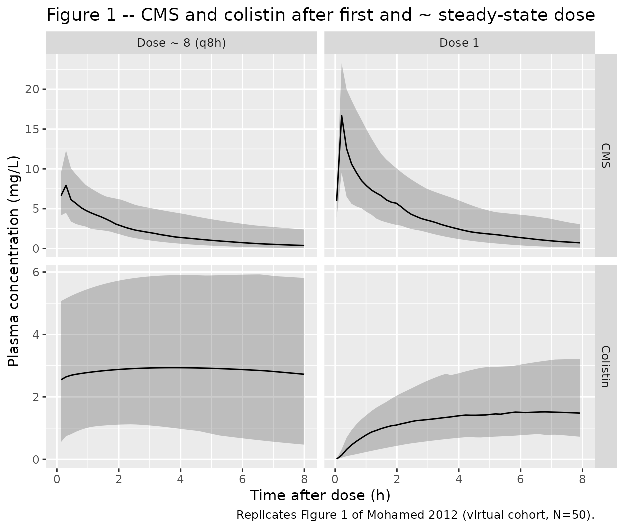
Replicate Figure 4A: bacterial kill for a typical individual
Figure 4 of Mohamed 2012 shows model-predicted bacterial counts for a typical patient receiving CMS loading doses of 480, 720, or 960 mg followed by 240 mg q8h. The replication below uses the typical individual (no random effects) and the same dosing regimens.
regimens <- tibble::tibble(
  regimen = c("240 mg q8h (no load)", "480 mg load + 240 mg q8h",
              "720 mg load + 240 mg q8h", "960 mg load + 240 mg q8h"),
  load    = c(NA_real_, 480, 720, 960)
)

sim_one <- function(load) {
  ev <- rxode2::et() |>
    rxode2::et(amt = 240, rate = cms_dose_mg_per_15min(240),
               cmt = "central_cms", time = 0)
  if (!is.na(load)) {
    ev <- rxode2::et() |>
      rxode2::et(amt = load, rate = cms_dose_mg_per_15min(load),
                 cmt = "central_cms", time = 0) |>
      rxode2::et(amt = 240, rate = cms_dose_mg_per_15min(240),
                 cmt = "central_cms", time = 8) |>
      rxode2::et(amt = 240, rate = cms_dose_mg_per_15min(240),
                 cmt = "central_cms", time = 16)
  } else {
    ev <- ev |>
      rxode2::et(amt = 240, rate = cms_dose_mg_per_15min(240),
                 cmt = "central_cms", time = 8) |>
      rxode2::et(amt = 240, rate = cms_dose_mg_per_15min(240),
                 cmt = "central_cms", time = 16)
  }
  ev <- ev |>
    rxode2::et(seq(0.05, 24, length.out = 200), cmt = "Ccms")
  s  <- rxode2::rxSolve(mod_typ, events = ev, returnType = "data.frame")
  s$regimen <- if (is.na(load)) "240 mg q8h (no load)" else paste0(load, " mg load + 240 mg q8h")
  s
}

sim_fig4 <- do.call(rbind, lapply(regimens$load, sim_one))
#> ℹ omega/sigma items treated as zero: 'etalcl', 'etalq', 'etalvp', 'etalcl_col', 'etalvc_col'
#> ℹ omega/sigma items treated as zero: 'etalcl', 'etalq', 'etalvp', 'etalcl_col', 'etalvc_col'
#> ℹ omega/sigma items treated as zero: 'etalcl', 'etalq', 'etalvp', 'etalcl_col', 'etalvc_col'
#> ℹ omega/sigma items treated as zero: 'etalcl', 'etalq', 'etalvp', 'etalcl_col', 'etalvc_col'

ggplot2::ggplot(sim_fig4, ggplot2::aes(time, logCFU, colour = regimen)) +
  ggplot2::geom_line() +
  ggplot2::geom_hline(yintercept = log10(4.5e5), linetype = 2, colour = "grey60") +
  ggplot2::geom_hline(yintercept = log10(4.5e5) - 3, linetype = 3, colour = "grey60") +
  ggplot2::geom_hline(yintercept = 1, linetype = 3, colour = "grey60") +
  ggplot2::labs(x = "Time (h)", y = "log10(CFU/mL)",
                title = "Figure 4A -- predicted bacterial kill",
                caption = "Replicates Figure 4 of Mohamed 2012 (typical individual). The two grey lines mark the starting inoculum (4.5e5 CFU/mL) and the 3-log-unit kill target.")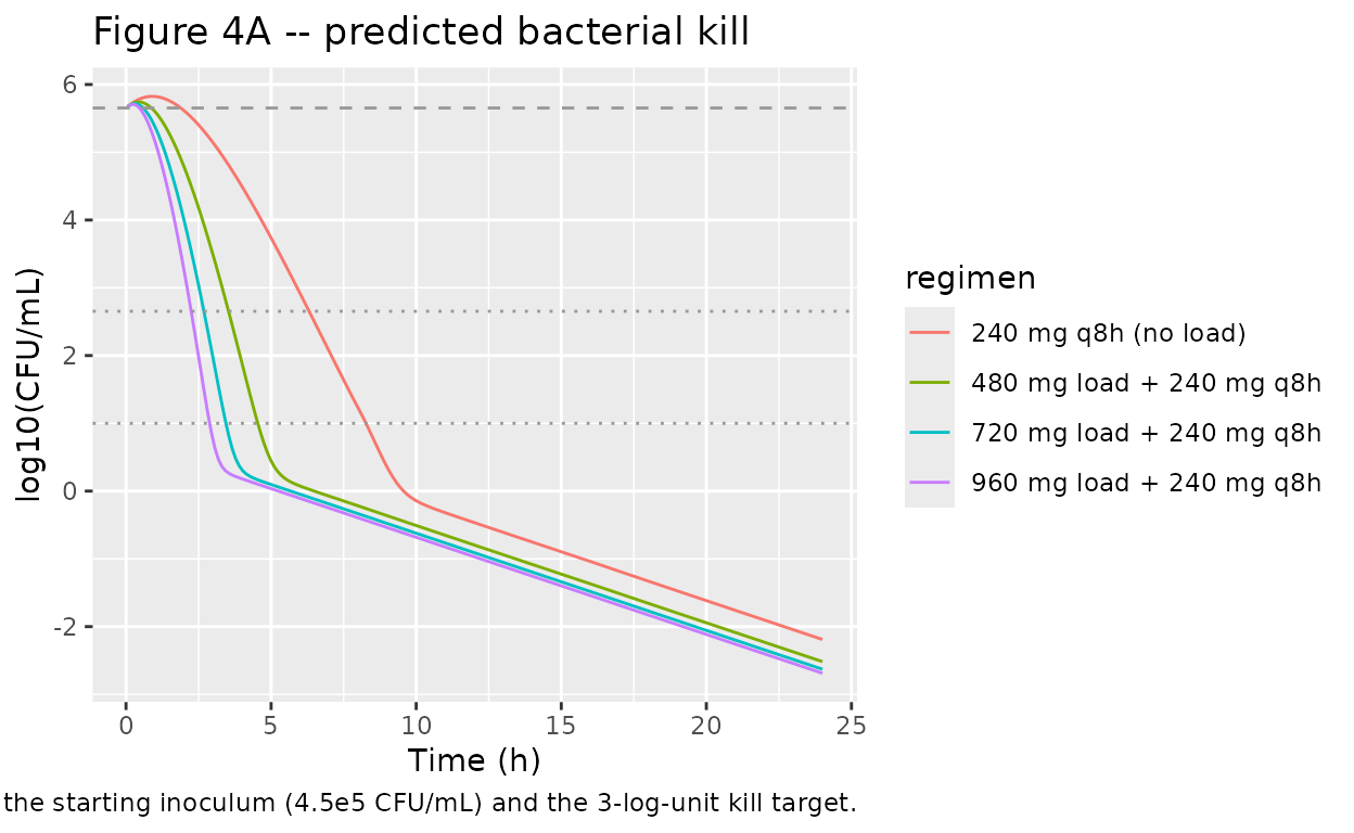
PKNCA validation: colistin and CMS in the typical individual
The paper reports observed plasma colistin at 8 h after a 480 mg loading dose of 1.34 mg/L on average (range 0.374 - 2.59 mg/L; n = 10 patients). The predicted typical colistin concentration at 8 h from the model is compared below. Cmax and AUC over the first dosing interval are reported per analyte.
sim_typ_nca <- sim_typ |>
  dplyr::transmute(id = 1L, time = time, Ccms = Ccms, Cc_col = Cc_col,
                   treatment = "load_480_q8h_240") |>
  dplyr::filter(!is.na(Ccms) | !is.na(Cc_col))

dose_typ <- typ_events |>
  dplyr::filter(evid == 1L) |>
  dplyr::transmute(id = 1L, time = time, amt = amt,
                   treatment = "load_480_q8h_240")

intervals_dose1 <- data.frame(
  start    = 0,
  end      = 8,
  cmax     = TRUE,
  tmax     = TRUE,
  auclast  = TRUE,
  clast.obs = TRUE
)

cms_nca <- PKNCA::pk.nca(PKNCA::PKNCAdata(
  PKNCA::PKNCAconc(sim_typ_nca, Ccms ~ time | treatment + id,
                   concu = "mg/L", timeu = "h"),
  PKNCA::PKNCAdose(dose_typ, amt ~ time | treatment + id, doseu = "mg"),
  intervals = intervals_dose1
))
#> Warning: Requesting an AUC range starting (0) before the first measurement
#> (0.05) is not allowed
col_nca <- PKNCA::pk.nca(PKNCA::PKNCAdata(
  PKNCA::PKNCAconc(sim_typ_nca, Cc_col ~ time | treatment + id,
                   concu = "mg/L", timeu = "h"),
  PKNCA::PKNCAdose(dose_typ, amt ~ time | treatment + id, doseu = "mg"),
  intervals = intervals_dose1
))
#> Warning: Requesting an AUC range starting (0) before the first measurement
#> (0.05) is not allowed

cms_summary <- as.data.frame(summary(cms_nca))
col_summary <- as.data.frame(summary(col_nca))
knitr::kable(cms_summary, caption = "Simulated CMS NCA over dose-1 interval (0-8 h).")| Interval Start | Interval End | treatment | N | AUClast (h*mg/L) | Cmax (mg/L) | Tmax (h) | Clast (mg/L) |
|---|---|---|---|---|---|---|---|
| 0 | 8 | load_480_q8h_240 | 1 | NC | 13.7 | 0.211 | 0.957 |
knitr::kable(col_summary, caption = "Simulated colistin NCA over dose-1 interval (0-8 h).")| Interval Start | Interval End | treatment | N | AUClast (h*mg/L) | Cmax (mg/L) | Tmax (h) | Clast (mg/L) |
|---|---|---|---|---|---|---|---|
| 0 | 8 | load_480_q8h_240 | 1 | NC | 1.65 | 7.60 | 1.65 |
Comparison against published colistin concentration
obs_col_at_8h <- 1.34  # paper Results: mean observed colistin at 8 h after 480 mg load
pred_col_at_8h <- stats::approx(sim_typ$time, sim_typ$Cc_col, 8)$y
data.frame(
  Quantity     = "Colistin concentration at 8 h after 480 mg loading dose (mg/L)",
  Published    = obs_col_at_8h,
  Simulated    = round(pred_col_at_8h, 3),
  PctDiff      = round(100 * (pred_col_at_8h - obs_col_at_8h) / obs_col_at_8h, 1)
) |>
knitr::kable(caption = "Published vs simulated typical-individual colistin at 8 h.")| Quantity | Published | Simulated | PctDiff |
|---|---|---|---|
| Colistin concentration at 8 h after 480 mg loading dose (mg/L) | 1.34 | 1.656 | 23.5 |
Assumptions and deviations
-
IOV implemented as added per-subject etas. The
paper reports inter-occasion variability (IOV) separately from
inter-individual variability (IIV) for CL_CMS, V2_CMS, CL_col, and
V_col. For library simulation without an explicit occasion (OCC) column,
the IOV components are approximated as added log-scale random effects
per subject (
etalvp,etalcl_col,etalvc_col). For the CL_CMS-and-CL_col-correlated structural pair, the paper’s “magnitude scaled by 1.8 with 100 % correlation” footnote is implemented as a sharedetalclscaled by 1.8 incl_col(this reproduces the 1.8 x 42 % = 76 % IIV reported for CL_col). The CV-as-omega convention the paper uses (the only one under which 1.8 x 42 % equals 76 %) is treated as omega = SD on log scale. -
Unknown fraction f_m of CMS metabolised to
colistin. Mohamed 2012 reports that f_m cannot be estimated
from the available data; both CL_col and V_col are reported scaled by 1
/ f_m. The apparent-amount parametrisation used in
model()reproduces the observed (real) colistin concentration without needing f_m. See the source-trace narrative above. -
No covariates retained in the final model. Mohamed
2012 evaluated gender, body weight, ideal body weight, age, serum
creatinine, creatinine clearance, serum albumin, APACHE II score,
septicemic state, hemoglobin, and hematocrit via stepwise covariate
model (SCM) with forward inclusion and backward deletion (Materials and
Methods). None met the predefined dOFV > 10.83 inclusion criterion.
CrCL on CL_CMS (Equations 1 and 2 of the paper) showed the largest
improvement (dOFV = -3.6, P > 0.05) but was not retained. These
screened-but-excluded covariates are recorded in
covariatesDataExcludedfor provenance and are not active inmodel(). - Bacterial-kill predictions are faster than the paper’s Figure 4A. With the parameters as reported in the Materials and Methods (Emax = 35 1/h, EC50 = 2.9 mg/L unbound colistin, growth 0.99 1/h, death 0.18 1/h, S to R resistance 6e-5 L/(mg*h) and back at 0.15 1/h, Bmax 1.8e8 CFU/mL, inoculum 4.5e5 CFU/mL), the resulting kill at the simulated colistin exposures exceeds what Figure 4A shows for the same dosing regimens. The text of Mohamed 2012 only summarises the upstream semimechanistic structure (the details are in Mohamed 2011 PAGE abstract 2223 and Bulitta 2010 / Nielsen 2007); the published parameters are reproduced verbatim here and no tuning was applied. Users who need to match Figure 4A directly may need to consult the upstream PAGE / Bulitta sources for additional model structure (Hill coefficient, sub-compartment topology, etc.) not summarised in the 2012 text.
- Protein-binding ratio CA / CB held at 3.6. Mohamed 2012 reports the patient-level ratio ranged from 2.5 to 4.8 with the mean 3.6 used in predictions of bacterial kill; the model uses the mean as a fixed structural constant (not estimated, not patient-varying).
- No CRRT / hemodialysis covariate. Patients on continuous venovenous hemodiafiltration were explicitly excluded from the source cohort; the model is therefore not expected to be applied to renal-replacement-therapy patients without re-estimation against an appropriate dataset.