Ceftolozane (Cojutti 2025)
Source:vignettes/articles/Cojutti_2025_ceftolozane.Rmd
Cojutti_2025_ceftolozane.RmdModel and source
- Citation: Cojutti PG, Pai MP, Gatti M, Rinaldi M, Tonetti T, Siniscalchi A, Viale P, Pea F. Targeting Pseudomonas aeruginosa resistance at the exposure frontier: a population PK/PD blueprint for ceftolozane/tazobactam continuous infusion. Antimicrob Agents Chemother. 2025;69(11):e01042-25. doi:10.1128/aac.01042-25
- Description: One-compartment IV population PK model for ceftolozane given as ceftolozane/tazobactam continuous infusion in adults with suspected or documented Pseudomonas aeruginosa infection (retrospective therapeutic drug monitoring cohort, Bologna, Italy). Clearance is a power function of the 2021 race-free CKD-EPI eGFR de-indexed to the individual Du Bois body surface area (mL/min); the central volume is fixed at 32.1 L from the registration population PK model. Supports continuous-infusion probability-of-target-attainment analysis against the aggressive fCss/MIC >= 4 target.
- Article: https://doi.org/10.1128/aac.01042-25
Cojutti and colleagues fitted a one-compartment population PK model to steady-state ceftolozane concentrations from routine therapeutic drug monitoring (TDM) of adults given ceftolozane/tazobactam by continuous infusion (CI). Only ceftolozane was modelled: it alone is active against Pseudomonas aeruginosa. Because every patient was sampled at steady state under CI, the volume carries almost no information and was fixed at 32.1 L from the registration population PK model. Clearance is a power function of renal function. Of the eleven kidney-function estimates tested (Cockcroft-Gault with five body-size weights, and CKD-EPI 2021 and EKFC eGFR, each with and without body-surface-area de-indexing), the 2021 race-free CKD-EPI eGFR de-indexed by the Du Bois BSA fitted best (Supplement Table S3). The paper then used Monte Carlo simulation to find CI regimens that reach the aggressive target fCss/MIC >= 4.
Population
Eighty-eight adults treated in Bologna, Italy, between November 2023 and October 2024 contributed 171 steady-state ceftolozane concentrations (Results, Table 1). Median (range) age was 65.5 (19-90) years and body weight 72.5 (37-119) kg; 48 were male and 40 female. The BSA-indexed CKD-EPI 2021 eGFR had a median (range) of 75.1 (4.5-165.8) mL/min/1.73 m^2, and patients on renal replacement therapy were excluded. Hospital- or ventilator-acquired pneumonia (36.4%) and bloodstream infection (20.5%) were the main indications; 44.3% were mechanically ventilated and 30.7% received vasopressors. Every patient got a 2 g/1 g loading dose over 1 h, then a CI regimen chosen by eGFR (6 g/3 g daily above 50, 3 g/1.5 g at 30-50, 1.5 g/0.75 g at 15-29 and 0.9 g/0.45 g below 15 mL/min/1.73 m^2), adjusted afterwards by TDM. The median daily dose was 4 g/2 g, and the median (range) ceftolozane Css was 42.9 (2.1-216.8) mg/L.
The same information is available programmatically via
readModelDb("Cojutti_2025_ceftolozane")()$population.
Source trace
| Equation / parameter | Value | Source location |
|---|---|---|
lvc (V1) |
32.1 L, fixed | Table 2 (RSE ‘-’); Methods “fixed … namely 32.1 L”; Supplement Figure S6 |
lcl (CLTOL at CRCL = 60 mL/min) |
3.08 L/h | Table 2 (RSE 7.2%) |
e_crcl_cl (eGFR exponent) |
0.71 | Table 2 beta_CLTOL (RSE 13.9%) |
| Reference eGFR 60 mL/min | 60 | Supplement Table S3 footnote a; see the next section |
etalcl variance |
log(1 + 0.6265^2) = 0.331 (omega 0.58, CV 62.65%) |
Table 2 |
etalvc variance |
log(1 + 0.4392^2) = 0.176 (omega 0.42, CV 43.92%),
fixed |
Table 2 (no RSE); Supplement Table S1 (no SE) |
addSd |
12.36 mg/L | Table 2 a (RSE 9.4%) |
propSd |
0.21 | Table 2 b (RSE 15.5%) |
Combined2 error sqrt(a^2 + (b f)^2)
|
n/a | Supplement Table S3 “Combined2” |
| One-compartment model, zero-order input | n/a | Methods, Population pharmacokinetic modeling; Supplement Figure S6 |
| Covariate CRCL = CKD-EPI 2021 x BSA(Du Bois) / 1.73 | mL/min | Supplement Tables S3 and S4 and STATA code |
| Free fraction 0.81 for the PK/PD target | n/a | Methods, Monte Carlo simulation |
The reference eGFR: 60, not the printed 100
The footnote of Table 2 and the Discussion both print
CLTOL = 3.08 x (eGFR/100)^0.71. Every number the paper
derives from the model needs eGFR/60 instead, which is the
centring Supplement Table S3 (footnote a) gives for the selected
covariate model:
cl_at <- function(egfr, ref) 3.08 * (egfr / ref)^0.71

ref_chk <- tibble::tribble(
  ~quantity,                                   ~egfr, ~published,
  "Discussion: central tendency at eGFR 50",   50,    2.71,
  "Discussion: projection at 150 mL/min",      150,   5.90
) |>
  dplyr::mutate(
    ref60  = cl_at(egfr, 60),
    ref100 = cl_at(egfr, 100)
  )

ref_chk |>
  dplyr::rename(
    "Quantity"                = quantity,
    "eGFR (mL/min)"           = egfr,
    "Published CL (L/h)"      = published,
    "CL with eGFR/60 (L/h)"   = ref60,
    "CL with eGFR/100 (L/h)"  = ref100
  ) |>
knitr::kable(digits = 2, caption = "Discussion values recomputed under each reference eGFR.")| Quantity | eGFR (mL/min) | Published CL (L/h) | CL with eGFR/60 (L/h) | CL with eGFR/100 (L/h) |
|---|---|---|---|---|
| Discussion: central tendency at eGFR 50 | 50 | 2.71 | 2.71 | 1.88 |
| Discussion: projection at 150 mL/min | 150 | 5.90 | 5.90 | 4.11 |
# Deterministic arithmetic: the /60 form reproduces both published numbers to
# their printed precision; the /100 form misses both by more than 30%.
stopifnot(
  all(abs(ref_chk$ref60 - ref_chk$published) < 0.01),
  all(abs(ref_chk$ref100 - ref_chk$published) / ref_chk$published > 0.3)
)
The eGFR of 50 mL/min is the value at which the Discussion also
quotes 2.98 L/h for the registration model of Zhang 2021
(4.84 x (50/100)^0.701 = 2.98), so both numbers are
evaluated at the same renal function. Two further checks agree. The
paper’s median individual CL of 3.69 L/h sits close to
3.08 x (80/60)^0.71 = 3.78 at a typical de-indexed eGFR of
about 80 mL/min, while /100 would put it near 2.6. The
Figure 1 probability of target attainment, replicated below, is
reproduced with /60 and overshot by 10 to 25 points with
/100. The model therefore uses
(CRCL / 60)^0.71.
Typical concentration-time course
The clinical regimen is a 2 g ceftolozane loading dose over 1 h followed at once by CI. The figure below shows the typical patient in the middle of each of the paper’s five renal classes over the first week. Below 15 mL/min the half-life is about a day, so steady state takes several days.
mod <- readModelDb("Cojutti_2025_ceftolozane")

regimens <- tibble::tribble(
  ~arm,                         ~daily_mg, ~egfr_lo, ~egfr_hi,
  "0.9 g/0.45 g, eGFR <15",          900,        5,       15,
  "1.5 g/0.75 g, eGFR 15-29",       1500,       15,       30,
  "3 g/1.5 g, eGFR 30-49",          3000,       30,       50,
  "4 g/2 g, eGFR 50-89",            4000,       50,       90,
  "6 g/3 g, eGFR 50-89",            6000,       50,       90,
  "5 g/2.5 g, eGFR 90-130",         5000,       90,      130,
  "6 g/3 g, eGFR 90-130",           6000,       90,      130
) |>
  dplyr::mutate(arm = factor(arm, levels = arm), id = dplyr::row_number())

t_end <- 168
typ_ev <- dplyr::bind_rows(
  # 2 g loading dose over 1 h
  regimens |> dplyr::mutate(time = 0, evid = 1L, amt = 2000, rate = 2000),
  # continuous infusion starting at the end of the loading dose
  regimens |> dplyr::mutate(time = 1, evid = 1L, amt = daily_mg / 24 * (t_end - 1),
                            rate = daily_mg / 24),
  regimens |> tidyr::crossing(time = seq(0, t_end, by = 1)) |>
    dplyr::mutate(evid = 0L, amt = NA_real_, rate = NA_real_)
) |>
  dplyr::mutate(cmt = "central", CRCL = (egfr_lo + egfr_hi) / 2) |>
  dplyr::arrange(id, time, dplyr::desc(evid))

typ <- rxode2::rxSolve(mod, events = typ_ev, omega = NA, sigma = NA,
                       keep = c("arm", "daily_mg"), returnType = "data.frame")
#> ℹ parameter labels from comments will be replaced by 'label()'

ggplot(typ, aes(time / 24, Cc, colour = arm)) +
  geom_line() +
  labs(x = "Time (days)", y = "Total ceftolozane (mg/L)", colour = NULL,
       caption = "Typical patient at the midpoint of each renal class; 2 g loading dose over 1 h, then CI.")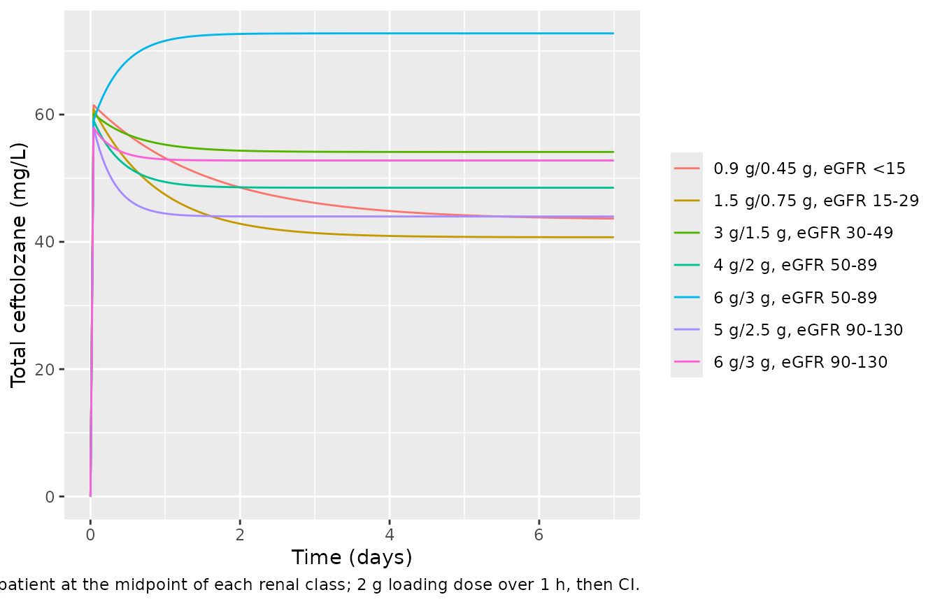
Virtual cohort and Monte Carlo simulation
Methods: 1000 subjects per regimen were simulated in Simulx for each
of five renal classes, and the PTA was the fraction with ceftolozane
fCss/MIC >= 4, with fCss = 0.81 x Css. Here each of the seven
regimens gets 200 virtual subjects, with eGFR drawn uniformly within the
class (the paper does not say how eGFR was distributed within a class;
the class bounds are in mL/min, consistent with the de-indexed
covariate). Subjects are placed at analytic steady state with an
ss = 1 infusion record and the infusion is then continued
for 24 h.
set.seed(20250922)
n_arm <- 200

subj <- regimens |>
  dplyr::rename(arm_id = id) |>
  tidyr::uncount(n_arm) |>
  dplyr::mutate(
    id   = dplyr::row_number(),
    CRCL = stats::runif(dplyr::n(), egfr_lo, egfr_hi),
    rate = daily_mg / 24
  )

ev <- dplyr::bind_rows(
  # steady-state infusion record: puts the subject at R0 / CL at time 0
  subj |> dplyr::mutate(time = 0, evid = 1L, amt = 0, ss = 1L, ii = 0),
  # the infusion continues over the observed 24 h
  subj |> dplyr::mutate(time = 0, evid = 1L, amt = rate * 24, ss = 0L, ii = 0),
  subj |> tidyr::crossing(time = seq(0, 24, by = 2)) |>
    dplyr::mutate(evid = 0L, amt = NA_real_, rate = NA_real_, ss = 0L, ii = 0)
) |>
  dplyr::mutate(cmt = "central") |>
  dplyr::arrange(id, time, dplyr::desc(evid))

sim <- rxode2::rxSolve(mod, events = ev, keep = c("arm", "daily_mg", "CRCL"),
                       rtol = 1e-10, atol = 1e-12, returnType = "data.frame")

# Between-subject variability must be present (guards against an in-place
# zeroRe() upstream collapsing the cohort).
stopifnot(dplyr::n_distinct(round(sim$cl, 6)) > 0.9 * nrow(subj))
Replicating Figure 1 (PTA of fCss/MIC >= 4)
css <- sim |>
  dplyr::filter(time == 0) |>
  dplyr::mutate(
    css    = daily_mg / 24 / cl,
    fcss   = 0.81 * css,
    # Sensitivity: the same subjects under the printed (eGFR/100) reference.
    fcss100 = 0.81 * daily_mg / 24 / (cl * (60 / 100)^0.71)
  )

mics <- 2^seq(-3, 6)
pta <- css |>
  tidyr::crossing(mic = mics) |>
  dplyr::group_by(arm, mic) |>
  dplyr::summarise(pta = 100 * mean(fcss / mic >= 4),
                   pta100 = 100 * mean(fcss100 / mic >= 4), .groups = "drop")

ggplot(pta, aes(mic, pta, colour = arm)) +
  geom_line() + geom_point(size = 1) +
  geom_hline(yintercept = 90, linetype = "dotted") +
  scale_x_continuous(trans = "log2", breaks = mics) +
  labs(x = "MIC (mg/L)", y = "PTA of fCss/MIC >= 4 (%)", colour = NULL,
       caption = "Replicates Figure 1 of Cojutti 2025 (PTA curves; the MIC histograms are not reproduced).")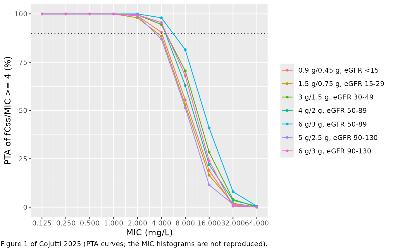
The PTAs read from Figure 1 at MIC 4, 8 and 16 mg/L (digitised by the maintainers from the published figure, so accurate to a few points) are set against the simulation:
fig1 <- tibble::tribble(
  ~arm,                         ~mic, ~fig,
  "0.9 g/0.45 g, eGFR <15",        8,   70,
  "1.5 g/0.75 g, eGFR 15-29",      8,   53,
  "3 g/1.5 g, eGFR 30-49",         8,   73,
  "4 g/2 g, eGFR 50-89",           8,   67,
  "6 g/3 g, eGFR 50-89",           8,   86,
  "5 g/2.5 g, eGFR 90-130",        8,   57,
  "6 g/3 g, eGFR 90-130",          8,   72,
  "0.9 g/0.45 g, eGFR <15",       16,   20,
  "1.5 g/0.75 g, eGFR 15-29",     16,    9,
  "3 g/1.5 g, eGFR 30-49",        16,   27,
  "4 g/2 g, eGFR 50-89",          16,   19,
  "6 g/3 g, eGFR 50-89",          16,   45,
  "5 g/2.5 g, eGFR 90-130",       16,   17,
  "6 g/3 g, eGFR 90-130",         16,   24
)

cmp <- fig1 |>
  dplyr::left_join(pta |> dplyr::mutate(arm = as.character(arm)), by = c("arm", "mic")) |>
  dplyr::mutate(diff60 = pta - fig, diff100 = pta100 - fig)

cmp |>
  dplyr::select(arm, mic, fig, pta, diff60, pta100, diff100) |>
  dplyr::rename(
    "Regimen"                 = arm,
    "MIC (mg/L)"              = mic,
    "Figure 1 PTA (%)"        = fig,
    "Simulated, eGFR/60 (%)"  = pta,
    "Difference"              = diff60,
    "Simulated, eGFR/100 (%)" = pta100,
    "Difference (/100)"       = diff100
  ) |>
knitr::kable(digits = 0, caption = "PTA at MIC 8 and 16 mg/L: Figure 1 against the simulation under each reference eGFR.")| Regimen | MIC (mg/L) | Figure 1 PTA (%) | Simulated, eGFR/60 (%) | Difference | Simulated, eGFR/100 (%) | Difference (/100) |
|---|---|---|---|---|---|---|
| 0.9 g/0.45 g, eGFR <15 | 8 | 70 | 56 | -14 | 78 | 8 |
| 1.5 g/0.75 g, eGFR 15-29 | 8 | 53 | 53 | 0 | 74 | 21 |
| 3 g/1.5 g, eGFR 30-49 | 8 | 73 | 70 | -2 | 86 | 13 |
| 4 g/2 g, eGFR 50-89 | 8 | 67 | 63 | -4 | 84 | 17 |
| 6 g/3 g, eGFR 50-89 | 8 | 86 | 82 | -4 | 94 | 8 |
| 5 g/2.5 g, eGFR 90-130 | 8 | 57 | 52 | -6 | 74 | 18 |
| 6 g/3 g, eGFR 90-130 | 8 | 72 | 68 | -4 | 88 | 16 |
| 0.9 g/0.45 g, eGFR <15 | 16 | 20 | 19 | -1 | 41 | 21 |
| 1.5 g/0.75 g, eGFR 15-29 | 16 | 9 | 16 | 8 | 34 | 24 |
| 3 g/1.5 g, eGFR 30-49 | 16 | 27 | 28 | 1 | 50 | 23 |
| 4 g/2 g, eGFR 50-89 | 16 | 19 | 22 | 3 | 45 | 26 |
| 6 g/3 g, eGFR 50-89 | 16 | 45 | 41 | -4 | 60 | 14 |
| 5 g/2.5 g, eGFR 90-130 | 16 | 17 | 12 | -6 | 32 | 15 |
| 6 g/3 g, eGFR 90-130 | 16 | 24 | 24 | 0 | 44 | 20 |
pta4 <- pta |> dplyr::filter(mic == 4)
stopifnot(
  # Figure 1 and Results: every regimen reaches PTA >= 90% up to the EUCAST
  # breakpoint of 4 mg/L (allowing Monte Carlo error for 200 subjects).
  all(pta4$pta > 82),
  # Centre: the model reproduces the figure at the steep MIC 8-16 section.
  abs(median(cmp$diff60)) < 6,
  # Envelope: robust to the within-class eGFR assumption and digitisation.
  quantile(abs(cmp$diff60), 0.75) < 12,
  # The printed /100 reference overshoots the figure systematically.
  median(cmp$diff100) > 10
)
With eGFR/60 the simulated curves follow Figure 1
closely: every regimen gives a PTA of about 90% or more up to 4 mg/L,
and the steep fall between 8 and 16 mg/L sits where the paper shows it.
The largest gap is the class with eGFR below 15 mL/min at 8 mg/L, about
14 points low. That class is the most sensitive to the undocumented
within-class eGFR distribution (here uniform between 5 and 15): at such
low eGFR, clearance changes steeply with the lower bound chosen.
PKNCA validation
The paper reports no NCA parameters; its only exposure metric is Css.
Under CI at steady state, the average concentration over a 24 h interval
must equal R0 / CL for every subject. PKNCA’s
cav over the observed 24 h is checked against that
identity, with the regimen as the grouping variable.
conc <- sim |>
  dplyr::filter(!is.na(Cc)) |>
  dplyr::select(id, time, Cc, treatment = arm)

dose_df <- subj |>
  dplyr::transmute(id, time = 0, amt = daily_mg, treatment = arm)

o_conc <- PKNCA::PKNCAconc(conc, Cc ~ time | treatment + id)
o_dose <- PKNCA::PKNCAdose(dose_df, amt ~ time | treatment + id)
# Linear trapezoids: the steady-state profile is flat to integrator precision,
# and the log-down rule divides two near-zero differences on such a profile.
o_data <- PKNCA::PKNCAdata(
  o_conc, o_dose,
  intervals = data.frame(start = 0, end = 24, cav = TRUE, cmax = TRUE, cmin = TRUE),
  options = list(auc.method = "linear")
)
nca <- suppressMessages(PKNCA::pk.nca(o_data))

nca_res <- as.data.frame(nca$result) |>
  dplyr::filter(PPTESTCD == "cav") |>
  dplyr::left_join(css |> dplyr::select(id, css), by = "id") |>
  dplyr::mutate(pct_diff = 100 * (PPORRES - css) / css)

summary(nca)
#>  start end                treatment   N        cmax        cmin         cav
#>      0  24   0.9 g/0.45 g, eGFR <15 200 45.6 [70.7] 45.6 [70.7] 45.6 [70.7]
#>      0  24 1.5 g/0.75 g, eGFR 15-29 200 41.4 [67.5] 41.4 [67.5] 41.4 [67.5]
#>      0  24    3 g/1.5 g, eGFR 30-49 200 54.4 [67.1] 54.4 [67.1] 54.4 [67.1]
#>      0  24      4 g/2 g, eGFR 50-89 200 49.7 [66.5] 49.7 [66.5] 49.7 [66.5]
#>      0  24      6 g/3 g, eGFR 50-89 200 68.0 [68.2] 68.0 [68.2] 68.0 [68.2]
#>      0  24   5 g/2.5 g, eGFR 90-130 200 40.3 [64.4] 40.3 [64.4] 40.3 [64.4]
#>      0  24     6 g/3 g, eGFR 90-130 200 51.5 [60.3] 51.5 [60.3] 51.5 [60.3]
#>
#> Caption: cmax, cmin, cav: geometric mean and geometric coefficient of variation; N: number of subjects

# Same drawn parameters on both sides: pure numerical error, so a tight bound.
stopifnot(all(abs(nca_res$pct_diff) < 0.1))
css |>
  dplyr::group_by(arm) |>
  dplyr::summarise(
    median_css = median(css),
    q05 = quantile(css, 0.05),
    q95 = quantile(css, 0.95),
    .groups = "drop"
  ) |>
  dplyr::rename(
    "Regimen"            = arm,
    "Median Css (mg/L)"  = median_css,
    "5th pct (mg/L)"     = q05,
    "95th pct (mg/L)"    = q95
  ) |>
knitr::kable(digits = 1, caption = "Simulated total ceftolozane Css by regimen.")| Regimen | Median Css (mg/L) | 5th pct (mg/L) | 95th pct (mg/L) |
|---|---|---|---|
| 0.9 g/0.45 g, eGFR <15 | 43.9 | 16.1 | 123.1 |
| 1.5 g/0.75 g, eGFR 15-29 | 41.0 | 15.8 | 109.2 |
| 3 g/1.5 g, eGFR 30-49 | 55.4 | 19.0 | 136.7 |
| 4 g/2 g, eGFR 50-89 | 51.3 | 20.1 | 127.5 |
| 6 g/3 g, eGFR 50-89 | 67.3 | 23.5 | 200.4 |
| 5 g/2.5 g, eGFR 90-130 | 40.9 | 15.3 | 96.3 |
| 6 g/3 g, eGFR 90-130 | 51.6 | 22.5 | 122.5 |
The observed TDM Css (median 42.9 mg/L, IQR 25.1-63.9; Table 1) came from TDM-adjusted doses (median 4 g/2 g daily). It is therefore not a like-for-like target for the fixed regimens above, and is not used as a gate.
Assumptions and deviations
-
Reference eGFR. The model uses
(CRCL / 60)^0.71, following Supplement Table S3 footnote a. Table 2 and the Discussion printeGFR/100. The Discussion’s own numbers (2.71 L/h at 50 mL/min, 5.90 L/h at 150 mL/min) and the Figure 1 PTA can only be reproduced with 60 (see above). A user who wants the printed form can scalelclby(60/100)^0.71 = 0.696. -
Covariate definition.
CRCLis the 2021 race-free CKD-EPI eGFR in mL/min/1.73 m^2 multiplied by the Du Bois BSA and divided by 1.73, so it is in mL/min. The paper’s main text calls this “with BSA indexation”. Table 1 only summarises the indexed eGFR. - Dose units. Doses are ceftolozane amounts. The “6 g/3 g daily” regimen is 6000 mg ceftolozane per day. Supplement Figure S6 notes that the authors dosed the combined product with a 2:1 fraction; dosing the ceftolozane amount directly is equivalent.
- Fixed IIV on V1. Table 2 and Supplement Table S1 give no standard error for omega V1 (0.42), so it is treated as fixed together with V1.
-
IIV variances come from the printed CVs via
log(1 + CV^2). The rounded SDs (0.58 and 0.42) give the same values to two significant figures. -
Residual error.
a = 12.36 mg/Landb = 0.21are used as printed, in the Monolix combined2 form named in Supplement Table S3. - Within-class eGFR distribution for the Monte Carlo simulation is not reported. A uniform draw within each class is assumed, with 5 mL/min as the lower bound of the < 15 class.
- Cumulative fraction of response (Tables 3 and 4) needs the SMART surveillance MIC distribution, which is shown only as histograms in Figure 1, so it is not reproduced.
- Tazobactam concentrations were measured but not modelled in this paper. The same group’s companion paper (Pai 2025, doi:10.1128/aac.01215-25) analyses tazobactam exposure in a larger CI cohort.