Piperacillin (Merino-Bohorquez 2021)
Source:vignettes/articles/MerinoBohorquez_2021_piperacillin.Rmd
MerinoBohorquez_2021_piperacillin.RmdModel and source
- Citation: Merino-Bohorquez V, Docobo-Perez F, Valiente-Mendez A, Delgado-Valverde M, Camean M, Hope WW, Pascual A, Rodriguez-Bano J. Population Pharmacokinetics of Piperacillin in Non-Critically Ill Patients with Bacteremia Caused by Enterobacteriaceae. Antibiotics (Basel). 2021;10(4):348. doi:10.3390/antibiotics10040348. PMCID: PMC8064303. Structural and variability estimates are Table 2; the structural equation is Equation (1); the residual-error polynomial is Methods 4.4. No supplementary material beyond the article figures was deposited.
- Description: One-compartment population PK model for intravenous piperacillin (given as piperacillin-tazobactam 4/0.5 g) in hospitalized, non-critically ill adults with Enterobacteriaceae bloodstream infection in Seville, Spain. Fitted non-parametrically with the NPAG algorithm in Pmetrics. Clearance is ADDITIVE in a covariate-free intercept and an arm linear in Cockcroft-Gault creatinine clearance expressed in L/h (paper: CL = Intercept + Slope x ClCr); the central volume carries no covariate. Every parameter carries inter-individual variability reconstructed as a log-normal from the mean and SD of the NPAG support-point distribution. Residual error is the published Pmetrics assay-error polynomial SD = 0.4388 + 0.027 x C (combined1), carried with the unreported gamma multiplier at 1. Merino-Bohorquez 2021, n = 27 subjects, 102 samples.
- Article: https://doi.org/10.3390/antibiotics10040348 (open access, PMC8064303)
No supplementary material beyond the article figures was deposited, and no erratum or correction to the article was found (Europe PMC search, 2026-09-28).
Population
Twenty-seven hospitalized, non-critically ill adults (not admitted to intensive care) with monomicrobial Enterobacteriaceae bloodstream infection, treated with piperacillin-tazobactam monotherapy at Hospital Universitario Virgen Macarena, Seville, Spain, between October 2012 and February 2015 (Merino-Bohorquez 2021 Table 1 and Methods 4.1). Median age was 76.5 years (range 48-86) and 17 of 27 (63%) were male; 79% had a body-mass index of at least 25 kg/m^2. The median Cockcroft-Gault creatinine clearance was 50.7 mL/min. The urinary tract was the most common source of bacteremia (67%), and Escherichia coli (15) and Klebsiella spp. (9) the most common organisms.
Patients received piperacillin-tazobactam 4/0.5 g by 4 h extended infusion every 8 h, with or without a preceding 30 min loading infusion of 4/0.5 g; patients with creatinine clearance below 20 mL/min/1.73 m^2 received the dose every 12 h. Four serum samples per patient were drawn at steady state, 1, 4, 6 and 8 h after the start of an infusion (102 samples in total, none below the 1 mg/L quantification limit).
The same information is available programmatically via
readModelDb("MerinoBohorquez_2021_piperacillin")()$population.
Source trace
The per-parameter origin is recorded as an in-file comment next to
each ini() entry in
inst/modeldb/specificDrugs/MerinoBohorquez_2021_piperacillin.R.
The table below collects them in one place.
| Equation / parameter | Value | Source location |
|---|---|---|
One-compartment structure,
dX1/dt = R(1) - ((Intercept + Slope x ClCr)/Vc) x X1
|
– | Results 2.2, Equation (1) |
CL = Intercept + Slope x ClCr, ClCr in L/h |
– | Table 2 row heading; Equation (1) |
lcl_nonren (Intercept) |
log(4.556) L/h |
Table 2, mean (SD 5.035, median 3.503) |
lcl_renal (Slope) |
log(1.353) |
Table 2, mean (SD 1.032, median 1.39) |
lvc (Vc) |
log(30.68) L |
Table 2, mean (SD 23.349, median 20.039) |
etalcl_nonren |
0.798104 | Table 2, log((5.035/4.556)^2 + 1)
|
etalcl_renal |
0.458555 | Table 2, log((1.032/1.353)^2 + 1)
|
etalvc |
0.456916 | Table 2, log((23.349/30.68)^2 + 1)
|
addSd (assay C0) |
fixed(0.4388) mg/L |
Methods 4.4, SD = gamma x (0.4388 + 0.027 x C)
|
propSd (assay C1) |
fixed(0.027) |
Methods 4.4 (same polynomial) |
CrCl conversion CRCL * 60 / 1000
|
mL/min to L/h | Table 1 unit (mL/min) and Table 2 unit (L/h) |
| Unbound fraction 0.7 (simulation only) | 0.7 | Methods 4.5 |
Typical-value checks
At the cohort median creatinine clearance of 50.7 mL/min (3.042 L/h)
the typical clearance is 4.556 + 1.353 x 3.042 = 8.67 L/h.
The first check solves the typical-value model and confirms that
clearance, and confirms that the creatinine-clearance arm is live: the
same model at CRCL = 0 must fall back to the intercept
alone.
mod <- rxode2::rxode2(readModelDb("MerinoBohorquez_2021_piperacillin"))
#> ℹ parameter labels from comments will be replaced by 'label()'
mod_typ <- rxode2::zeroRe(mod)

crcl_levels <- c(0, 20, 50.7, 110)
ev_typ <- do.call(
  rbind,
  lapply(seq_along(crcl_levels), function(i) {
    dose <- data.frame(
      id = i, time = seq(0, 40, by = 8), amt = 4000, rate = 1000, evid = 1
    )
    obs <- data.frame(
      id = i, time = seq(0, 48, by = 0.1), amt = 0, rate = 0, evid = 0
    )
    out <- dplyr::bind_rows(dose, obs)
    out$CRCL <- crcl_levels[i]
    out
  })
) |>
  dplyr::mutate(cmt = "central") |>
  dplyr::arrange(id, time, dplyr::desc(evid))

# zeroRe() sets the omegas to zero, so rxode2 warns that a multi-subject
# simulation has no omega; for typical-value solves that is the intent.
solve_typical <- function(model, events) {
  withCallingHandlers(
    suppressMessages(rxode2::rxSolve(model, events, returnType = "data.frame")),
    warning = function(w) {
      if (grepl("omega", conditionMessage(w))) invokeRestart("muffleWarning")
    }
  )
}
sim_typ <- solve_typical(mod_typ, ev_typ) |>
  dplyr::mutate(treatment = paste0("CRCL ", crcl_levels[id], " mL/min"))

cl_typ <- sim_typ |>
  dplyr::group_by(id, treatment) |>
  dplyr::summarise(cl = dplyr::first(cl), .groups = "drop") |>
  dplyr::mutate(
    CRCL = crcl_levels[id],
    cl_expected = 4.556 + 1.353 * CRCL * 60 / 1000
  )
knitr::kable(
  cl_typ |>
    dplyr::select(treatment, cl, cl_expected) |>
    dplyr::rename(
      "Creatinine clearance" = treatment,
      "Model CL (L/h)" = cl,
      "Table 2 CL (L/h)" = cl_expected
    ),
  digits = 3
)| Creatinine clearance | Model CL (L/h) | Table 2 CL (L/h) |
|---|---|---|
| CRCL 0 mL/min | 4.556 | 4.556 |
| CRCL 20 mL/min | 6.180 | 6.180 |
| CRCL 50.7 mL/min | 8.672 | 8.672 |
| CRCL 110 mL/min | 13.486 | 13.486 |
stopifnot(
  # Same drawn parameters on both sides: a tight numerical bound is correct.
  all(abs(cl_typ$cl - cl_typ$cl_expected) < 1e-8),
  # The creatinine-clearance arm must move clearance.
  cl_typ$cl[cl_typ$CRCL == 110] > 2 * cl_typ$cl[cl_typ$CRCL == 0]
)
The 4 g, 4 h infusion every 8 h regimen is at steady state well
before the sixth dose (the typical half-life at 50.7 mL/min is
log(2) x 30.68 / 8.67 = 2.45 h). The PKNCA analysis of the
40-48 h interval gives AUCtau, which must equal
Dose / CL for every renal-function group.
ggplot(dplyr::filter(sim_typ, time >= 24), aes(time, Cc, colour = treatment)) +
  geom_line() +
  labs(x = "Time (h)", y = "Total piperacillin (mg/L)", colour = NULL) +
  theme_bw()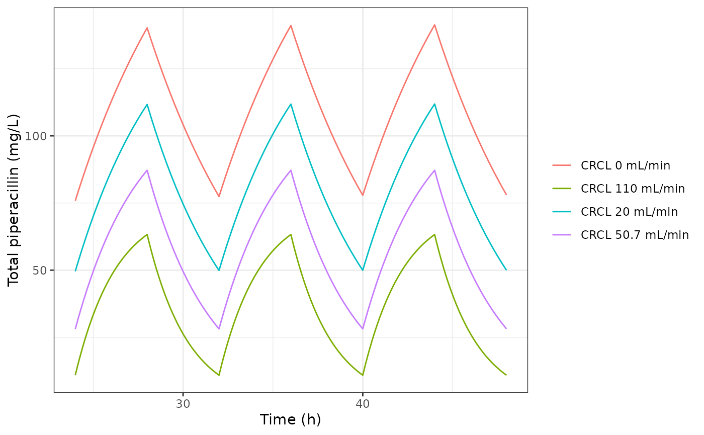
Typical-value steady-state profiles for 4 g piperacillin by 4 h infusion every 8 h at four creatinine clearances.
conc_df <- sim_typ |>
  dplyr::filter(!is.na(Cc)) |>
  dplyr::select(id, treatment, time, Cc)
dose_df <- ev_typ |>
  dplyr::filter(evid == 1) |>
  dplyr::mutate(treatment = paste0("CRCL ", crcl_levels[id], " mL/min")) |>
  dplyr::select(id, treatment, time, amt)

o_conc <- PKNCA::PKNCAconc(conc_df, Cc ~ time | treatment + id)
o_dose <- PKNCA::PKNCAdose(dose_df, amt ~ time | treatment + id)
intervals <- data.frame(start = 40, end = 48, auclast = TRUE, cmax = TRUE, cmin = TRUE)
nca_res <- PKNCA::pk.nca(PKNCA::PKNCAdata(o_conc, o_dose, intervals = intervals))

nca_wide <- as.data.frame(nca_res) |>
  dplyr::select(treatment, PPTESTCD, PPORRES) |>
  tidyr::pivot_wider(names_from = PPTESTCD, values_from = PPORRES) |>
  dplyr::left_join(dplyr::select(cl_typ, treatment, cl), by = "treatment") |>
  dplyr::mutate(auc_x_cl = auclast * cl)

knitr::kable(
  nca_wide |>
    dplyr::rename(
      "Creatinine clearance" = treatment,
      "Cmax,ss (mg/L)" = cmax,
      "Cmin,ss (mg/L)" = cmin,
      "AUCtau (mg*h/L)" = auclast,
      "CL (L/h)" = cl,
      "AUCtau x CL (mg)" = auc_x_cl
    ),
  digits = 2
)| Creatinine clearance | AUCtau (mg*h/L) | Cmax,ss (mg/L) | Cmin,ss (mg/L) | CL (L/h) | AUCtau x CL (mg) |
|---|---|---|---|---|---|
| CRCL 0 mL/min | 876.99 | 141.30 | 77.87 | 4.56 | 3995.58 |
| CRCL 110 mL/min | 296.59 | 63.25 | 10.90 | 13.49 | 3999.74 |
| CRCL 20 mL/min | 647.22 | 111.84 | 49.96 | 6.18 | 3999.55 |
| CRCL 50.7 mL/min | 461.25 | 87.17 | 28.14 | 8.67 | 3999.87 |
# Steady-state identity AUCtau x CL = Dose (4000 mg); the residual is
# trapezoidal error on a 0.1 h grid.
stopifnot(all(abs(nca_wide$auc_x_cl / 4000 - 1) < 0.005))
The paper reports no NCA summary, so there is no published NCA table to compare against. For orientation, the observed concentrations in Figure 1 span roughly 1-250 mg/L, which brackets the typical steady-state profiles above.
Replicating Table 3: probability of target attainment
Table 3 reports the probability of attaining unbound concentrations
above the MIC for at least 50% of the first 24 h
(fT>MIC >= 50%) for six regimens, with an unbound
fraction fixed at 0.7 (Methods 4.5):
- Normal renal function (90-129 mL/min/1.73 m^2): Dosage 1, 4 g (0.5 h infusion) q8h; Dosage 2, 4 g (4 h infusion) q8h; Dosage 3, 4 g (0.5 h) followed immediately by 4 g (4 h), then 4 g (4 h) q8h.
- Severely decreased renal function or kidney failure (< 30 mL/min/1.73 m^2): Dosages 4-6, the same three patterns every 12 h.
The simulation below uses 200 virtual patients per renal-function group, with creatinine clearance drawn uniformly across the group’s band. To make the result reproducible across rxode2 builds, the random effects are drawn with base R and passed to the typical-value model as data columns, so rxode2 draws no random numbers. Each renal-function group uses one set of patients for all three of its regimens.
om <- diag(mod$omega)
n_per_arm <- 200

draw_cohort <- function(crcl_lo, crcl_hi, seed) {
  set.seed(seed)
  data.frame(
    id = seq_len(n_per_arm),
    CRCL = stats::runif(n_per_arm, crcl_lo, crcl_hi),
    etalcl_nonren = stats::rnorm(n_per_arm, 0, sqrt(om[["etalcl_nonren"]])),
    etalcl_renal = stats::rnorm(n_per_arm, 0, sqrt(om[["etalcl_renal"]])),
    etalvc = stats::rnorm(n_per_arm, 0, sqrt(om[["etalvc"]]))
  )
}

regimen_doses <- function(pattern, tau) {
  starts <- seq(0, 47, by = tau)
  if (pattern == "short") {
    data.frame(time = starts, amt = 4000, rate = 4000 / 0.5)
  } else if (pattern == "extended") {
    data.frame(time = starts, amt = 4000, rate = 4000 / 4)
  } else {
    # Loading: 0.5 h infusion, then the 4 h infusion starting immediately
    # after it (Methods 4.2), repeated every tau from that start.
    dplyr::bind_rows(
      data.frame(time = 0, amt = 4000, rate = 4000 / 0.5),
      data.frame(time = starts + 0.5, amt = 4000, rate = 4000 / 4)
    )
  }
}

simulate_regimen <- function(cohort, pattern, tau, model) {
  dose <- regimen_doses(pattern, tau)
  dose$evid <- 1
  obs <- data.frame(time = seq(0, 48, by = 0.1), amt = 0, rate = 0, evid = 0)
  events <- merge(cohort, dplyr::bind_rows(dose, obs)) |>
    dplyr::mutate(cmt = "central") |>
    dplyr::arrange(id, time, dplyr::desc(evid))
  # The eta columns in the data supply each subject's random effects.
  solve_typical(model, events)
}

regimens <- data.frame(
  dosage = 1:6,
  group = rep(c("normal", "renal"), each = 3),
  pattern = rep(c("short", "extended", "loading"), 2),
  tau = rep(c(8, 12), each = 3)
)
cohorts <- list(
  normal = draw_cohort(90, 129, seed = 20210325),
  renal = draw_cohort(5, 29, seed = 20210326)
)

run_all <- function(model) {
  do.call(
    rbind,
    lapply(seq_len(nrow(regimens)), function(i) {
      r <- regimens[i, ]
      s <- simulate_regimen(cohorts[[r$group]], r$pattern, r$tau, model)
      s$dosage <- r$dosage
      s[, c("dosage", "id", "time", "Cc")]
    })
  )
}
sim_pta <- run_all(mod_typ)

mics <- c(0.06, 0.125, 0.25, 0.5, 1, 2, 4, 8, 16, 32, 64, 128, 256)
pta_table <- function(sim) {
  ft <- sim |>
    dplyr::filter(time < 24) |>
    dplyr::group_by(dosage, id)
  do.call(
    rbind,
    lapply(mics, function(m) {
      ft |>
        dplyr::summarise(ft = mean(0.7 * Cc > m), .groups = "drop") |>
        dplyr::group_by(dosage) |>
        dplyr::summarise(pta = 100 * mean(ft >= 0.5), .groups = "drop") |>
        dplyr::mutate(mic = m)
    })
  )
}
pta_sim <- pta_table(sim_pta)
# Table 3 of Merino-Bohorquez 2021, transcribed by column (Dosage 1-6).
pta_paper <- data.frame(
  mic = rep(mics, 6),
  dosage = rep(1:6, each = length(mics)),
  pta_paper = c(
    c(99.8, 99.2, 99, 98.8, 98.4, 97.4, 93.4, 76.4, 56.8, 14.2, 1.2, 0, 0),
    c(100, 100, 100, 100, 100, 100, 100, 100, 95.8, 28, 2, 0, 0),
    c(100, 100, 100, 100, 100, 100, 100, 100, 94.6, 45.8, 8.4, 0.2, 0),
    c(99.4, 99.2, 99.2, 99.2, 98.9, 98.8, 98.5, 92.9, 77.3, 38.7, 6.9, 1.2, 0.2),
    c(99.9, 99.9, 99.9, 99.8, 99.7, 99.6, 99.5, 96.1, 90.7, 61.1, 11.7, 1.2, 0.2),
    c(100, 100, 100, 100, 100, 100, 99.9, 99.7, 94.3, 81.3, 31.8, 4.6, 0.7)
  )
)
pta_cmp <- dplyr::left_join(pta_paper, pta_sim, by = c("mic", "dosage"))

knitr::kable(
  pta_cmp |>
    dplyr::mutate(col = paste0("Dosage ", dosage, " paper / sim")) |>
    dplyr::mutate(val = sprintf("%.1f / %.1f", pta_paper, pta)) |>
    dplyr::select(mic, col, val) |>
    tidyr::pivot_wider(names_from = col, values_from = val) |>
    dplyr::rename("MIC (mg/L)" = mic),
  caption = "Replicates Table 3 of Merino-Bohorquez 2021: PTA (%) for fT>MIC >= 50% over 0-24 h, published / simulated."
)| MIC (mg/L) | Dosage 1 paper / sim | Dosage 2 paper / sim | Dosage 3 paper / sim | Dosage 4 paper / sim | Dosage 5 paper / sim | Dosage 6 paper / sim |
|---|---|---|---|---|---|---|
| 0.060 | 99.8 / 95.5 | 100.0 / 100.0 | 100.0 / 100.0 | 99.4 / 98.5 | 99.9 / 100.0 | 100.0 / 100.0 |
| 0.125 | 99.2 / 94.0 | 100.0 / 100.0 | 100.0 / 100.0 | 99.2 / 98.0 | 99.9 / 100.0 | 100.0 / 100.0 |
| 0.250 | 99.0 / 93.5 | 100.0 / 100.0 | 100.0 / 100.0 | 99.2 / 97.5 | 99.9 / 100.0 | 100.0 / 100.0 |
| 0.500 | 98.8 / 92.0 | 100.0 / 100.0 | 100.0 / 100.0 | 99.2 / 97.0 | 99.8 / 100.0 | 100.0 / 100.0 |
| 1.000 | 98.4 / 91.0 | 100.0 / 100.0 | 100.0 / 100.0 | 98.9 / 94.0 | 99.7 / 99.5 | 100.0 / 100.0 |
| 2.000 | 97.4 / 87.5 | 100.0 / 100.0 | 100.0 / 100.0 | 98.8 / 92.0 | 99.6 / 98.5 | 100.0 / 99.0 |
| 4.000 | 93.4 / 83.0 | 100.0 / 100.0 | 100.0 / 100.0 | 98.5 / 89.5 | 99.5 / 97.5 | 99.9 / 98.0 |
| 8.000 | 76.4 / 73.0 | 100.0 / 98.5 | 100.0 / 100.0 | 92.9 / 83.0 | 96.1 / 91.5 | 99.7 / 94.5 |
| 16.000 | 56.8 / 53.0 | 95.8 / 83.5 | 94.6 / 92.0 | 77.3 / 63.5 | 90.7 / 78.5 | 94.3 / 88.0 |
| 32.000 | 14.2 / 14.0 | 28.0 / 27.0 | 45.8 / 46.5 | 38.7 / 35.5 | 61.1 / 40.0 | 81.3 / 63.5 |
| 64.000 | 1.2 / 1.0 | 2.0 / 1.5 | 8.4 / 3.5 | 6.9 / 6.0 | 11.7 / 5.5 | 31.8 / 24.5 |
| 128.000 | 0.0 / 0.0 | 0.0 / 0.0 | 0.2 / 0.0 | 1.2 / 0.0 | 1.2 / 0.0 | 4.6 / 1.0 |
| 256.000 | 0.0 / 0.0 | 0.0 / 0.0 | 0.0 / 0.0 | 0.2 / 0.0 | 0.2 / 0.0 | 0.7 / 0.0 |
ggplot(pta_cmp, aes(mic, colour = factor(dosage))) +
  geom_line(aes(y = pta)) +
  geom_point(aes(y = pta_paper)) +
  scale_x_continuous(trans = "log2", breaks = mics, labels = mics) +
  facet_wrap(~ ifelse(dosage <= 3, "Normal renal function (q8h)", "Severe impairment / failure (q12h)")) +
  labs(x = "MIC (mg/L)", y = "PTA (%)", colour = "Dosage") +
  theme_bw() +
  theme(axis.text.x = element_text(angle = 45, hjust = 1))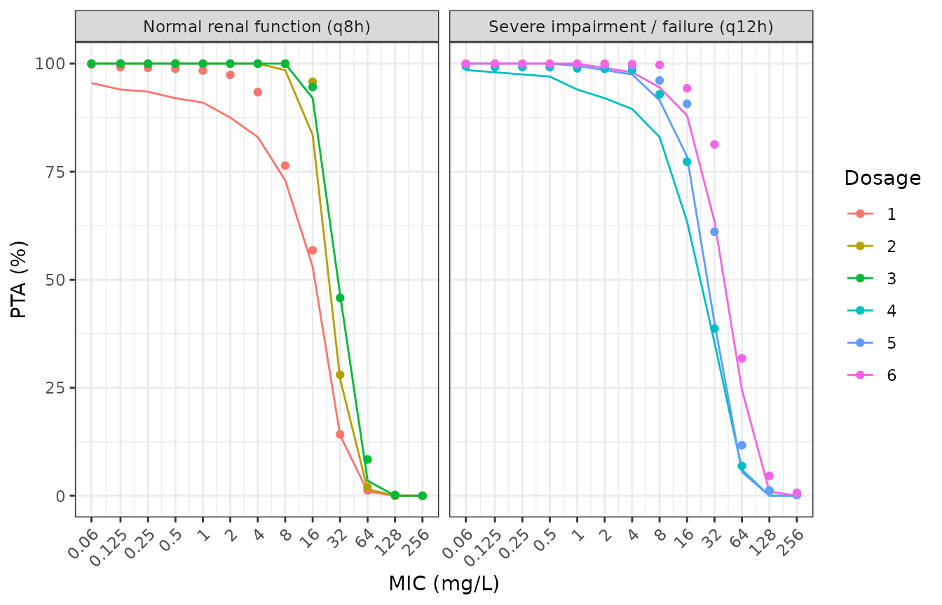
Replicates Table 3 of Merino-Bohorquez 2021. Points: published PTA; lines: simulated from the packaged model.
The summary statistic compared across the six regimens is the MIC at which the PTA falls through 50% (log2-interpolated between the bracketing dilutions). It depends on the typical clearance and volume and on the regimen, so a mis-transcribed parameter, a wrong creatinine-clearance scale or a wrong infusion duration moves it by more than one dilution.
mic50 <- function(mic, pta) {
  i <- which(pta[-length(pta)] >= 50 & pta[-1] < 50)[1]
  l2 <- log2(mic)
  2^(l2[i] + (pta[i] - 50) / (pta[i] - pta[i + 1]) * (l2[i + 1] - l2[i]))
}
mic50_cmp <- pta_cmp |>
  dplyr::arrange(dosage, mic) |>
  dplyr::group_by(dosage) |>
  dplyr::summarise(
    mic50_paper = mic50(mic, pta_paper),
    mic50_sim = mic50(mic, pta),
    .groups = "drop"
  ) |>
  dplyr::mutate(log2_ratio = log2(mic50_sim / mic50_paper))
knitr::kable(
  mic50_cmp |>
    dplyr::rename(
      "Dosage" = dosage,
      "MIC at 50% PTA, paper (mg/L)" = mic50_paper,
      "MIC at 50% PTA, simulated (mg/L)" = mic50_sim,
      "log2(simulated / paper)" = log2_ratio
    ),
  digits = 2
)| Dosage | MIC at 50% PTA, paper (mg/L) | MIC at 50% PTA, simulated (mg/L) | log2(simulated / paper) |
|---|---|---|---|
| 1 | 17.87 | 16.88 | -0.08 |
| 2 | 25.55 | 24.13 | -0.08 |
| 3 | 30.15 | 30.34 | 0.01 |
| 4 | 26.12 | 22.35 | -0.23 |
| 5 | 37.39 | 26.73 | -0.48 |
| 6 | 49.60 | 40.68 | -0.29 |
stopifnot(
  # Every regimen within one doubling dilution of the published PTA curve.
  all(abs(mic50_cmp$log2_ratio) < 1),
  # Extended infusion beats the short infusion in both renal-function groups,
  # as the paper reports.
  mic50_cmp$mic50_sim[2] > mic50_cmp$mic50_sim[1],
  mic50_cmp$mic50_sim[5] > mic50_cmp$mic50_sim[4]
)
The simulated curves reproduce the ranking and position of the published ones, but they sit at or below Table 3: the 50%-PTA MIC is -0.08, -0.08, 0.01, -0.23, -0.48, -0.29 doublings from the paper for Dosages 1-6, and at the lowest MICs the short-infusion arms lose a few percent of patients that the paper does not. That is the expected consequence of replacing the paper’s non-parametric 13-support-point density with independent log-normal marginals whose CVs are 76-111% (see Assumptions and deviations): the log-normal tails contain patients with very high clearance and very small volume that a bounded support-point mixture does not.
Sensitivity: typical value taken as the NPAG mean vs. a moment-matched log-normal
The packaged model uses each Table 2 mean as the median of its
log-normal marginal, the convention of the other Pmetrics models in
nlmixr2lib. That places the simulated population MEAN above the
published mean (by a factor sqrt(1 + CV^2), i.e. 1.49 for
the intercept and 1.26 for the slope and Vc). The alternative is to
choose the log-normal median so that the population mean and SD both
match Table 2. This section reports the 50%-PTA MIC under that
alternative; it is shown for interpretation only and does not change the
packaged model.
cv <- c(5.035 / 4.556, 1.032 / 1.353, 23.349 / 30.68)
theta_mm <- c(4.556, 1.353, 30.68) / sqrt(1 + cv^2)
mod_mm <- rxode2::ini(
  mod_typ,
  lcl_nonren = log(theta_mm[1]),
  lcl_renal = log(theta_mm[2]),
  lvc = log(theta_mm[3])
)
#> ℹ change initial estimate of `lcl_nonren` to `1.11739294109386`
#> ℹ change initial estimate of `lcl_renal` to `0.0730468283904774`
#> ℹ change initial estimate of `lvc` to `3.19515291895853`
pta_mm <- pta_table(run_all(mod_mm))
mic50_mm <- dplyr::left_join(pta_paper, pta_mm, by = c("mic", "dosage")) |>
  dplyr::arrange(dosage, mic) |>
  dplyr::group_by(dosage) |>
  dplyr::summarise(mic50_mm = mic50(mic, pta), .groups = "drop")
knitr::kable(
  dplyr::left_join(mic50_cmp, mic50_mm, by = "dosage") |>
    dplyr::select(dosage, mic50_paper, mic50_sim, mic50_mm) |>
    dplyr::rename(
      "Dosage" = dosage,
      "Paper (mg/L)" = mic50_paper,
      "Packaged model (mg/L)" = mic50_sim,
      "Moment-matched log-normal (mg/L)" = mic50_mm
    ),
  digits = 2,
  caption = "MIC at which PTA falls through 50%, by typical-value encoding."
)| Dosage | Paper (mg/L) | Packaged model (mg/L) | Moment-matched log-normal (mg/L) |
|---|---|---|---|
| 1 | 17.87 | 16.88 | 21.02 |
| 2 | 25.55 | 24.13 | 31.49 |
| 3 | 30.15 | 30.34 | 40.82 |
| 4 | 26.12 | 22.35 | 33.19 |
| 5 | 37.39 | 26.73 | 38.42 |
| 6 | 49.60 | 40.68 | 57.81 |
mic50_both <- dplyr::left_join(mic50_cmp, mic50_mm, by = "dosage")
stopifnot(
  # Lower log-normal medians mean lower clearance and larger MICs covered.
  all(mic50_both$mic50_mm > mic50_both$mic50_sim)
)
The moment-matched alternative moves every curve to higher MICs, by 0.04 to 0.44 doublings from the paper, against -0.48 to 0.01 for the packaged model. Neither log-normal encoding reproduces Table 3 uniformly, which is expected when the underlying population distribution is a discrete support-point mixture.
Toxicodynamic thresholds
Methods 4.6 evaluates unbound trough concentrations on day 2 against a neurotoxicity threshold of 157.2 mg/L (and 361.4 mg/L) and a nephrotoxicity threshold of 452.65 mg/L. The paper reports that none of the normal-renal-function patients and 0.2-0.3% of the renally impaired patients on extended or loading regimens exceeded 157.2 mg/L. With 200 virtual patients per group, one patient is 0.5%, so the simulation can only confirm that exceedances are rare.
tox <- sim_pta |>
  dplyr::filter(time >= 24, time <= 48) |>
  dplyr::group_by(dosage, id) |>
  dplyr::summarise(cmin_u = min(0.7 * Cc), .groups = "drop") |>
  dplyr::group_by(dosage) |>
  dplyr::summarise(
    `> 157.2 mg/L (%)` = 100 * mean(cmin_u > 157.2),
    `> 361.4 mg/L (%)` = 100 * mean(cmin_u > 361.4),
    `> 452.65 mg/L (%)` = 100 * mean(cmin_u > 452.65),
    `Median unbound Cmin (mg/L)` = stats::median(cmin_u),
    .groups = "drop"
  ) |>
  dplyr::rename("Dosage" = dosage)
knitr::kable(tox, digits = 1)| Dosage | > 157.2 mg/L (%) | > 361.4 mg/L (%) | > 452.65 mg/L (%) | Median unbound Cmin (mg/L) |
|---|---|---|---|---|
| 1 | 0 | 0 | 0 | 3.3 |
| 2 | 0 | 0 | 0 | 7.7 |
| 3 | 0 | 0 | 0 | 7.7 |
| 4 | 0 | 0 | 0 | 8.8 |
| 5 | 0 | 0 | 0 | 12.8 |
| 6 | 0 | 0 | 0 | 13.3 |
Assumptions and deviations
-
Non-parametric to parametric. The paper fitted the
model with the non-parametric NPAG algorithm in Pmetrics, whose
population distribution is a set of 13 support points (Methods 4.5).
That joint distribution is not published. Table 2 reports the mean, SD
and median of each marginal; the packaged model encodes each marginal as
a log-normal with median equal to the Table 2 mean and variance
log(CV^2 + 1)withCV = SD / mean, and treats the three random effects as independent. The intercept and slope of a linear clearance model are almost certainly correlated in the support points, and that correlation is lost. The paper’s own Monte Carlo draws (a multivariate normal around each support point with covariance divided by 13) cannot be reproduced. -
Mean vs. median. Table 2 prints both a mean and a
median. The mean was used as the typical value, consistent with the
other Pmetrics models in nlmixr2lib (for example
Sime_2019_tazobactamandTsai_2023_ceftriaxone). The medians (3.503 L/h, 1.39, 20.039 L) are recorded in the model file. For the slope the printed median exceeds the mean, so no single log-normal reproduces both summaries. -
Creatinine-clearance scale. Table 2 and Equation
(1) apply the slope to creatinine clearance in L/h, while Table 1
reports creatinine clearance in mL/min. The model therefore takes
CRCLin mL/min, as reported, and converts it internally. Reading the slope against mL/min would give a clearance of about 73 L/h at the cohort median, which is incompatible with both the observed concentrations in Figure 1 and the Table 3 target attainment. - Creatinine-clearance range. Table 1 prints a range of 45.3-255.3 mL/min, but Results 2.1 states that three patients had creatinine clearance below 20 mL/min/1.73 m^2. The printed minimum is inconsistent with the text; the model is used here, as in the paper, down to kidney failure, but the paper notes that few patients with severe impairment informed the fit.
- Renal-function bands in the simulations. The paper does not say how creatinine clearance was assigned within each KDIGO band. The simulation draws it uniformly over 90-129 mL/min (normal) and 5-29 mL/min (severely decreased or kidney failure), and treats the band limits (mL/min/1.73 m^2) as if they were Cockcroft-Gault values in mL/min.
- Loading-dose timing. Dosages 3 and 6 start the first 4 h infusion immediately after the 0.5 h loading infusion (Methods 4.2) and repeat it every 8 or 12 h from that start. The paper does not state whether the maintenance schedule is timed from the loading infusion or the first extended infusion.
-
Residual error. Pmetrics weights observations by
SD = gamma x (0.4388 + 0.027 x C)(Methods 4.4). The assay coefficients are fixed inputs and are wrapped infixed(). The estimatedgammais not reported, so the unscaled polynomial (gamma = 1) is carried, as inTsai_2023_ceftriaxone. Pmetrics adds the two terms linearly, which is nlmixr2’scombined1()form. None of the checks in this article uses the residual error. -
Unbound fraction. The paper’s target-attainment and
toxicity analyses use an unbound fraction of 0.7 (Methods 4.5, citing
the literature). It is not part of the fitted model, so the model’s
Ccis total piperacillin and the factor is applied in this article. -
Target-attainment window. PTA is evaluated over the
first 24 h of therapy, following the
fTMIC0-24hwording of the Table 3 caption.