Model and source
- Citation: Li C, Shoji S, Beebe J. Pharmacokinetics and C-reactive protein modelling of anti-interleukin-6 antibody (PF-04236921) in healthy volunteers and patients with autoimmune disease. Br J Clin Pharmacol. 2018;84(9):2059-2074. doi:10.1111/bcp.13641
- Description: Integrated population PK and indirect-response PK/PD model for the anti-interleukin-6 monoclonal antibody PF-04236921 in healthy volunteers and adults with rheumatoid arthritis, Crohn’s disease, or systemic lupus erythematosus (Li 2018). Two-compartment IV/SC PK with first-order absorption and linear elimination from the central compartment; disease-stratified linear clearance and PD parameters; PF-04236921 inhibits the zero-order CRP synthesis rate of an indirect-response model.
- Article: https://doi.org/10.1111/bcp.13641
PF-04236921 is a fully-human anti-interleukin-6 monoclonal antibody developed by Pfizer. The Li 2018 paper integrates pharmacokinetic and PK/PD data from five Phase 1 / Phase 2 trials covering healthy volunteers, rheumatoid arthritis, Crohn’s disease, and systemic lupus erythematosus into a single popPK and indirect-response PK/PD model on serum C-reactive protein (CRP).
Population
The pooled analysis dataset included 392 subjects across five clinical studies:
- B0151001 (Phase 1 single ascending IV dose, healthy volunteers, n = 36)
- B0151004 (Phase 1 single 200 mg SC dose, healthy volunteers, n = 10)
- B0151002 (Phase 1 multiple ascending IV dose, rheumatoid arthritis on background methotrexate, n = 31)
- B0151003 (Phase 2 proof-of-concept SC dose-ranging, moderate-to-severe Crohn’s disease refractory to anti-TNF, n = 178)
- B0151006 (Phase 2 proof-of-concept SC dose-ranging, active generalized systemic lupus erythematosus, n = 138)
Baseline demographics summarised from Li 2018 Table 2 (p2065): pooled-cohort median body weight 72 kg (range 30-157 kg), albumin 4.0 g/dL (2.3-5.0 g/dL), creatinine clearance 113 mL/min (47.0-329 mL/min), and baseline CRP varying across cohorts from a median of 0.9 mg/L in healthy volunteers to 19.4 mg/L in CD subjects. The pooled cohort is approximately 48 percent female.
The same population summary is available programmatically via
readModelDb("Li_2018_PF04236921")$population.
Source trace
In-file source-trace comments live next to every ini()
entry in inst/modeldb/specificDrugs/Li_2018_PF04236921.R.
The table below collects them in one place.
| Equation / parameter | Value | Source location |
|---|---|---|
lcl (HV reference CL) |
log(0.00546 L/h) | Table 3A theta_CL,HV (p2068) |
e_ra_cl, e_cd_cl,
e_sle_cl
|
log-ratios on HV CL | Table 3A theta_CL,RA/CD/SLE (p2068) |
lvc |
log(3.03 L) | Table 3A theta_Vc |
lq |
log(0.0245 L/h) | Table 3A theta_Q |
lvp |
log(3.58 L) | Table 3A theta_Vp |
lka |
log(0.00607 1/h) | Table 3A theta_ka |
lfdepot |
log(1) fixed | Results “Final PK model” p2063 (“F fixed to 100 percent”) |
e_wt_cl, e_wt_vc, e_wt_q,
e_wt_vp
|
power exponents | Table 3A theta_BWT_on_* (ref 72 kg, p2064 PK equation) |
e_alb_cl, e_crcl_cl,
e_crp_cl
|
power exponents | Table 3A (ref 4.0 g/dL ALB, 113 mL/min CRCL, 7.6 mg/L CRP) |
e_sex_cl |
0.862 multiplier | Table 3A theta_SEX_on_CL (paper Eq. (theta)^(SEX-1)) |
q_vc_scale |
2.73 | Table 3A theta_IIV_on_Q; paper Eq. eta_Q = theta * eta_Vc |
| IIV block (CL, Vc, Vp) | omega^2 = (CV/100)^2 | Table 3A footnote b on p2069 |
lbase, e_*_base
|
typical BLCRP per cohort | Table 3B theta_BLCRP,HV/RA/CD/SLE (p2068) |
e_alb_base |
-3.69 | Table 3B theta_ALB_on_BLCRP |
lic50, e_*_ic50
|
typical IC50 per cohort | Table 3B IC50,HV/RA/CD/SLE |
logitimax, e_*_logitimax
|
typical Imax per cohort | Table 3B Imax,HV/RA/CD/SLE (Imax = exp(theta_Imax)/(1 + exp(theta_Imax))) |
e_alb_logitimax |
-1.53 power exp (logit scale) | Table 3B theta_ALB_on_Imax |
lkout |
log(0.0238 1/h) | Table 3B theta_Kout |
lgamma |
log(1) fixed | Table 3B theta_gamma,HV/RA/CD = 1 fix |
e_sle_gamma |
log(1.55) | Table 3B theta_gamma,SLE |
| IIV block (BLCRP, Imax) + IC50 | omega^2 = (CV/100)^2 | Table 3B footnote d on p2069 |
PK residual expSd
|
0.179 | Table 3A pooled patient CV (RA/CD/SLE) |
PD residual expSd_CRP
|
0.453 | Table 3B residual CV (45.3 percent) |
| ODE: 2-cmt PK + first-order absorption | n/a | Results “Final PK model” p2063 + paper Eq. p2064 |
| ODE: indirect response on CRP | n/a | Methods “Final PK/PD model” p2062, p2066 |
Virtual cohort
The original observed concentrations are not publicly available. The
figures below use deterministic typical-value simulations from the
published parameter estimates (between-subject variability zeroed out
via rxode2::zeroRe()) running one representative dose level
per cohort.
Reference covariate values for the typical subject (Li 2018 Methods, p2064 and Supplemental Figure S3 caption): BWT 72 kg, ALB 4.0 g/dL, CRCL 113 mL/min, CRP 1.16 / 7.81 / 15.5 / 2.42 mg/L for HV / RA / CD / SLE respectively, male.
set.seed(2018)

mod_full <- rxode2::rxode2(readModelDb("Li_2018_PF04236921"))
#> ℹ parameter labels from comments will be replaced by 'label()'
mod_typ  <- rxode2::zeroRe(mod_full)

# Observation grid (in hours) -- 0 to 60 weeks
obs_times <- sort(unique(c(
  seq(0,   28,   by = 1),
  seq(28,  168,  by = 4),
  seq(168, 720,  by = 12),
  seq(720, 60 * 168, by = 24)
)))

make_cohort <- function(id, label, route, doses_mg, dose_times_h,
                        WT, SEXF, ALB, CRCL, CRP,
                        DIS_RA, DIS_CD, DIS_SLE) {
  cmt_dose <- if (route == "iv") "central" else "depot"
  ev <- rxode2::et()
  for (k in seq_along(doses_mg)) {
    ev <- rxode2::et(ev,
                     amt  = doses_mg[k],
                     cmt  = cmt_dose,
                     evid = 1L,
                     time = dose_times_h[k])
  }
  # Sample Cc at every time on the grid; sample CRP_pred at the same grid.
  ev <- rxode2::et(ev, obs_times, cmt = "Cc")
  ev <- rxode2::et(ev, obs_times, cmt = "CRP_pred")
  ev <- as.data.frame(ev)
  ev$id      <- id
  ev$cohort  <- label
  ev$WT      <- WT
  ev$SEXF    <- SEXF
  ev$ALB     <- ALB
  ev$CRCL    <- CRCL
  ev$CRP     <- CRP
  ev$DIS_RA  <- DIS_RA
  ev$DIS_CD  <- DIS_CD
  ev$DIS_SLE <- DIS_SLE
  ev
}

events <- bind_rows(
  make_cohort(1L, "HV-IV (700 mg single IV)",  "iv",
              doses_mg = 700,  dose_times_h = 0,
              WT = 72, SEXF = 0, ALB = 45, CRCL = 116, CRP = 9,
              DIS_RA = 0, DIS_CD = 0, DIS_SLE = 0),
  make_cohort(2L, "HV-SC (200 mg single SC)",  "sc",
              doses_mg = 200,  dose_times_h = 0,
              WT = 72, SEXF = 0, ALB = 45, CRCL = 123, CRP = 8,
              DIS_RA = 0, DIS_CD = 0, DIS_SLE = 0),
  make_cohort(3L, "RA-IV (250 mg IV Q4W x 3)", "iv",
              doses_mg = c(250, 250, 250),  dose_times_h = c(0, 28*24, 56*24),
              WT = 61, SEXF = 10, ALB = 42, CRCL = 93.3, CRP = 7.4,
              DIS_RA = 1, DIS_CD = 0, DIS_SLE = 0),
  make_cohort(4L, "CD-SC (200 mg SC at Day 1, Week 4)", "sc",
              doses_mg = c(200, 200),  dose_times_h = c(0, 4 * 7 * 24),
              WT = 70, SEXF = 10, ALB = 40, CRCL = 110, CRP = 19.4,
              DIS_RA = 0, DIS_CD = 1, DIS_SLE = 0),
  make_cohort(5L, "SLE-SC (200 mg SC at Day 1, Week 8, Week 16)", "sc",
              doses_mg = c(200, 200, 200),  dose_times_h = c(0, 8 * 7 * 24, 16 * 7 * 24),
              WT = 73, SEXF = 10, ALB = 39, CRCL = 119, CRP = 29,
              DIS_RA = 0, DIS_CD = 0, DIS_SLE = 1)
)
Simulation
sim <- rxode2::rxSolve(mod_typ, events = events, keep = c("cohort"))
#> ℹ omega/sigma items treated as zero: 'etalcl', 'etalvc', 'etalvp', 'etalka', 'etalbase', 'etalogitimax', 'etalic50'
#> Warning: multi-subject simulation without without 'omega'
sim_df <- as.data.frame(sim)
Replicate published figures
The published PK time courses (paper Figure 1a) show multi-exponential decay following the IV doses and a flatter SC profile reflecting the slow absorption rate (ka = 0.00607 1/h, absorption half-life ~ 5 days). The simulated typical profiles below reproduce that qualitative shape.
sim_df |>
  dplyr::filter(time > 0, Cc > 0) |>
  ggplot(aes(time / (24 * 7), Cc, colour = cohort)) +
  geom_line(linewidth = 0.6) +
  scale_y_log10() +
  labs(
    x = "Time (weeks)",
    y = "PF-04236921 concentration (ng/mL)",
    title = "Figure 1a-equivalent: typical-value PK by cohort",
    caption = "Replicates the qualitative dose-route stratification in Figure 1a of Li 2018."
  ) +
  theme_minimal() +
  theme(legend.position = "bottom")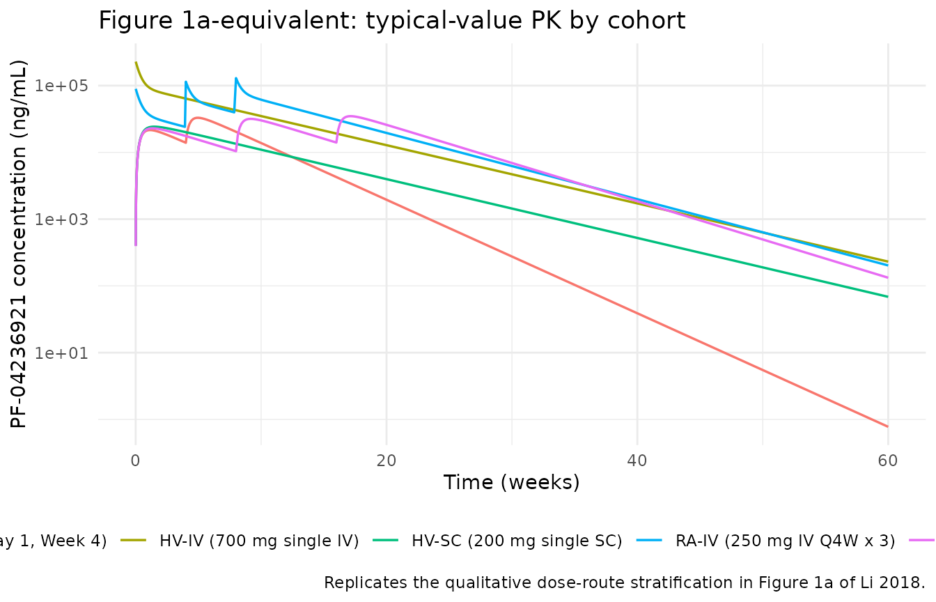
The published CRP response (paper Figure 1b) shows a delayed CRP reduction relative to PF-04236921 Cmax (the paper notes a ~5-day delay) followed by recovery as drug is cleared. Note: the CRP curve below uses the cohort-specific baseline CRP value as the steady-state pre-dose CRP (CRP(0) = BLCRP), and the simulated CRP returns toward that baseline after drug elimination.
sim_df |>
  ggplot(aes(time / (24 * 7), CRP_pred, colour = cohort)) +
  geom_line(linewidth = 0.6) +
  scale_y_log10() +
  labs(
    x = "Time (weeks)",
    y = "CRP (mg/L)",
    title = "Figure 1b-equivalent: typical-value CRP response by cohort",
    caption = "Replicates the qualitative CRP reduction pattern in Figure 1b of Li 2018."
  ) +
  theme_minimal() +
  theme(legend.position = "bottom")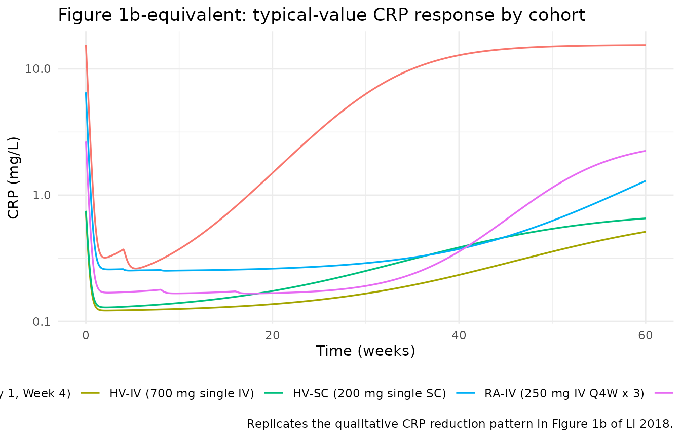
PKNCA validation
NCA for the single-dose cohorts (HV-IV 700 mg and HV-SC 200 mg). The multi-dose cohorts (RA, CD, SLE) accumulate concentration across dosing intervals and are not directly comparable to a single-dose NCA.
sim_nca <- sim_df |>
  dplyr::filter(time > 0, !is.na(Cc), Cc > 0,
                cohort %in% c("HV-IV (700 mg single IV)",
                              "HV-SC (200 mg single SC)")) |>
  dplyr::distinct(id, time, .keep_all = TRUE) |>
  dplyr::transmute(id = as.integer(id), time = time / 24, Cc = Cc, treatment = cohort)

dose_df <- events |>
  dplyr::filter(evid == 1, id %in% c(1L, 2L)) |>
  dplyr::transmute(id = as.integer(id), time = time / 24, amt = amt,
                   treatment = cohort)

conc_obj <- PKNCA::PKNCAconc(sim_nca, Cc ~ time | treatment + id)
dose_obj <- PKNCA::PKNCAdose(dose_df, amt ~ time | treatment + id)

intervals <- data.frame(
  start       = 0,
  end         = 60 * 7,  # day
  cmax        = TRUE,
  tmax        = TRUE,
  aucinf.obs  = TRUE,
  half.life   = TRUE
)

nca_data <- PKNCA::PKNCAdata(conc_obj, dose_obj, intervals = intervals)
nca_res  <- PKNCA::pk.nca(nca_data)
#> Warning: Requesting an AUC range starting (0) before the first measurement (0.0416667) is not allowed
#> Requesting an AUC range starting (0) before the first measurement (0.0416667) is not allowed
knitr::kable(
  as.data.frame(nca_res$result),
  caption = "Simulated NCA parameters for single-dose HV cohorts (time in days, Cc in ng/mL)."
)| treatment | id | start | end | PPTESTCD | PPORRES | exclude |
|---|---|---|---|---|---|---|
| HV-IV (700 mg single IV) | 1 | 0 | 420 | cmax | 2.288190e+05 | NA |
| HV-IV (700 mg single IV) | 1 | 0 | 420 | tmax | 4.166670e-02 | NA |
| HV-IV (700 mg single IV) | 1 | 0 | 420 | tlast | 4.200000e+02 | NA |
| HV-IV (700 mg single IV) | 1 | 0 | 420 | clast.obs | 1.191643e+02 | NA |
| HV-IV (700 mg single IV) | 1 | 0 | 420 | lambda.z | 1.594030e-02 | NA |
| HV-IV (700 mg single IV) | 1 | 0 | 420 | r.squared | 9.999017e-01 | NA |
| HV-IV (700 mg single IV) | 1 | 0 | 420 | adj.r.squared | 9.999015e-01 | NA |
| HV-IV (700 mg single IV) | 1 | 0 | 420 | lambda.z.time.first | 5.666667e+00 | NA |
| HV-IV (700 mg single IV) | 1 | 0 | 420 | lambda.z.time.last | 4.200000e+02 | NA |
| HV-IV (700 mg single IV) | 1 | 0 | 420 | lambda.z.n.points | 4.450000e+02 | NA |
| HV-IV (700 mg single IV) | 1 | 0 | 420 | clast.pred | 1.183644e+02 | NA |
| HV-IV (700 mg single IV) | 1 | 0 | 420 | half.life | 4.348396e+01 | NA |
| HV-IV (700 mg single IV) | 1 | 0 | 420 | span.ratio | 9.528419e+00 | NA |
| HV-IV (700 mg single IV) | 1 | 0 | 420 | aucinf.obs | NA | Requesting an AUC range starting (0) before the first measurement (0.0416667) is not allowed |
| HV-SC (200 mg single SC) | 2 | 0 | 420 | cmax | 2.384893e+04 | NA |
| HV-SC (200 mg single SC) | 2 | 0 | 420 | tmax | 1.000000e+01 | NA |
| HV-SC (200 mg single SC) | 2 | 0 | 420 | tlast | 4.200000e+02 | NA |
| HV-SC (200 mg single SC) | 2 | 0 | 420 | clast.obs | 3.558283e+01 | NA |
| HV-SC (200 mg single SC) | 2 | 0 | 420 | lambda.z | 1.603530e-02 | NA |
| HV-SC (200 mg single SC) | 2 | 0 | 420 | r.squared | 9.999851e-01 | NA |
| HV-SC (200 mg single SC) | 2 | 0 | 420 | adj.r.squared | 9.999851e-01 | NA |
| HV-SC (200 mg single SC) | 2 | 0 | 420 | lambda.z.time.first | 1.050000e+01 | NA |
| HV-SC (200 mg single SC) | 2 | 0 | 420 | lambda.z.time.last | 4.200000e+02 | NA |
| HV-SC (200 mg single SC) | 2 | 0 | 420 | lambda.z.n.points | 4.300000e+02 | NA |
| HV-SC (200 mg single SC) | 2 | 0 | 420 | clast.pred | 3.570735e+01 | NA |
| HV-SC (200 mg single SC) | 2 | 0 | 420 | half.life | 4.322633e+01 | NA |
| HV-SC (200 mg single SC) | 2 | 0 | 420 | span.ratio | 9.473393e+00 | NA |
| HV-SC (200 mg single SC) | 2 | 0 | 420 | aucinf.obs | NA | Requesting an AUC range starting (0) before the first measurement (0.0416667) is not allowed |
Comparison against published expectations
Li 2018 reports key descriptive PK metrics in the Results and Discussion rather than in a side-by-side single-dose NCA table:
- SC absorption peak: paper p2065 notes Cmax was reached at approximately 120 hours (5 days) post-dose following a single 200 mg SC administration in study B0151004; the simulated Tmax above for HV-SC should fall in the same range.
-
Terminal half-life: paper p2070 reports
approximately 32-39 days in healthy / RA / SLE subjects from the
beta-phase elimination rate constant; the simulated
half.lifefor HV-IV should fall in that range. - Dose-normalized AUCinf: paper p2065 reports geometric mean of 262,050 ng/h/mL per mg for SC 200 mg in B0151004. The simulated typical AUCinf for HV-SC divided by 200 mg gives a comparable reference value.
-
Per-cohort typical CRP: pre-dose typical CRP equals
the cohort-specific
BLCRPfrom Table 3B (1.16 / 7.81 / 15.5 / 2.42 mg/L for HV / RA / CD / SLE), and the simulated CRP_pred at time 0 should match these.
Assumptions and deviations
Residual error. Li 2018 estimated separate log-normal residual variance for HV.IV (CV 10.7 percent), HV.SC (CV 28.3 percent), and the pooled patient cohort RA/CD/SLE (CV 17.9 percent), with an additional IIV(eta_error) = 40.1 percent multiplying the per-subject residual SD on the PK side. The packaged model collapses this three-group residual structure to the pooled-patient single value (
expSd = 0.179) and drops the IIV-on-residual layer because nlmixr2’s log-normal error model assumes a single residual SD per output. The same simplification applies to the PD residual (singleexpSd_CRP = 0.453, no IIV-on-residual). Downstream simulations under the packaged model are slightly less variable than the paper’s NONMEM fits.Disease-cohort parameter encoding. The paper estimated
theta_CL,theta_BLCRP,theta_IC50, andtheta_Imaxseparately for each of the four cohorts (HV, RA, CD, SLE) as independent THETAs. The packaged model re-expresses this as a HV-reference structural value plus three log-shift covariate-effect parameters keyed onDIS_RA,DIS_CD, andDIS_SLE. The numerical typical values for each cohort match the paper’s Table 3A and Table 3B exactly when only one indicator is 1 (the cohorts are non-overlapping). The encoding is mathematically equivalent to the paper’s per-cohort THETAs but presents a cleaner covariate-effect interface.Imax covariate form. The paper’s Eq. (p2066) writes
theta_prime_Imax = theta_Imax * (ALB / 4.0)^theta_ALB_on_Imax, i.e. the ALB effect is multiplicative on the LOGIT-scale parameter rather than additive. The packaged model encodes this multiplicative form verbatim; it differs from the more common “additive on logit” convention. For ALB at the reference 4.0 g/dL the multiplier is 1 and the cohort-specific Imax matches the published value.Eta_Q derived from eta_Vc. The paper writes
eta_Q = theta_IIV_on_Q * eta_Vc(a derived random effect rather than an independent draw). The packaged model encodes this with a fixed-effect scalarq_vc_scale = 2.73applied toetalvcinside the Q parameterisation, matching the paper’s structural form. This avoids the singular 4x4 covariance matrix that would result from forcing eta_Q to be 100 percent correlated with eta_Vc inside the IIV block.CRP units. The covariate column
CRPand the model stateeffect(outputCRP_pred) are both in mg/L per the paper’s Table 2 reporting. The paper’s Methods section reports the LLOQ in mg/dL (1 mg/dL = 10 mg/L); this model file’s covariate notes flag the mg/L convention explicitly.Creatinine clearance units. Li 2018 Table 2 reports CLcr in “mL/min” without the BSA normalisation that the canonical
CRCLregister entry defaults to (mL/min/1.73 m^2). The packaged model carries the raw mL/min unit and documents the deviation incovariateData[[CRCL]]$notesso that a downstream user supplies the same convention.Bioavailability. SC F was fixed to 1 in the paper’s base model (Results, p2063), supported by comparable dose-normalised AUCinf estimates between IV and SC at similar doses. The packaged model encodes this as
lfdepot <- fixed(log(1)).Placebo / baseline drift. The paper found placebo-arm CRP time courses were approximately constant (Supplemental Figure S1) and the model assumes a constant pre-treatment CRP equal to BLCRP. No placebo / baseline-drift term is in the packaged model.
Typical-value figures vs VPCs. The published Figure 1 (panels a and b) shows observed-data medians and the published Figure 4 shows prediction-corrected VPCs. The reproductions in this vignette use the typical patient (random effects zeroed via
rxode2::zeroRe()) at one representative dose per cohort – enough to reproduce the qualitative dose-route stratification but not the within-cohort variability or the dose-range richness of the published figures.