Peg-IFN-alpha-induced HBsAg loss in chronic hepatitis B (Hanan 2026)
Source:vignettes/articles/Hanan_2026_peginterferon_alfa_hbsag_loss.Rmd
Hanan_2026_peginterferon_alfa_hbsag_loss.RmdModel and source
- Citation: Hanan NJ, Zierhut ML, Nader A, Mahajan A, Kaur A, Kumar K, Dixon SA, Das J, Magee M, Theodore D, Gielen V. A Systematic Review and Model-Based Meta-Analysis of Pegylated-Interferon-alpha-Induced HBsAg Loss in Chronic Hepatitis B Virus Infection. CPT Pharmacometrics Syst Pharmacol. 2026;15:e70164. doi:10.1002/psp4.70164.
- Article: https://doi.org/10.1002/psp4.70164 (Open Access; PMC12823784)
- Supplement (Data S1): PRISMA flow diagram (Figure S1) and the PICOS inclusion / exclusion table (Table S1). It contains no parameters; it contributed only population metadata to this extraction.
- Errata: none. Crossref
update-toandupdated-byare both null.
This paper contributes two model files, because the authors fit their two efficacy endpoints independently (Section 2.3) on different analysis sets with different retained covariates:
| Model file | Endpoint | Analysis set | Retained covariates |
|---|---|---|---|
Hanan_2026_peginterferon_alfa_eot_mbma |
HBsAg loss at end of treatment (EOT) | 45 studies / 52 strata / 83 study-strata-arms / 11,493 participants | duration, baseline HBsAg, HBeAg status |
Hanan_2026_peginterferon_alfa_24wk_mbma |
HBsAg loss 24 weeks after Peg-IFN-alpha cessation (functional-cure surrogate) | 28 studies / 35 strata / 58 study-strata-arms / 4,267 participants | duration, baseline HBsAg |
Baseline HBeAg status is the one structural difference between them: it is retained at end of treatment (OR 2.37) and screened-but-not-retained at 24 weeks. The 24-week model therefore predicts the same probability for HBeAg-positive and HBeAg-negative arms, and the EOT coefficient must not be carried over to it.
Why this is an extraction and not a systematic-review skip
Page 1 carries a “SYSTEMIC REVIEW” banner and the Methods describe a
PRISMA literature search of Embase / MEDLINE / Cochrane (January 2000 to
July 2022), so the systematic-review skip pathway applies to the
data collection step only. The literature search is how the
authors assembled their dataset; the model itself is original, fit by
the authors in R 4.2.1 with nlme, and Table 2 is their own
parameter table (logit-scale estimates, %RSE, 95% prediction intervals,
p-values, between-trial variance) rather than a catalogue of other
authors’ models.
Population
| Field | Value |
|---|---|
| Species | human |
| Disease state | chronic hepatitis B virus (HBV) infection |
| Participants (EOT / 24-week) | 11,493 / 4,267 |
| Studies (EOT / 24-week) | 45 / 28 |
| Study-strata-arms (EOT / 24-week) | 83 / 58 |
| Age | adults (Hanan 2026 Table S1 PICOS: age group ‘Adults’) |
| Regimens | standard Peg-IFNalpha regimens only (studies investigating non-standard Peg-IFNalpha dosing were excluded); Peg-IFNalpha monotherapy or Peg-IFNalpha + nucleos(t)ide analogue combination therapy |
The observation unit is the study-strata-arm: a treatment arm within a study, optionally stratified by HBeAg status, baseline HBsAg or baseline HBV DNA. The data are aggregate published results, not individual patient data, so every simulation in this vignette produces a study-arm mean proportion and none of it is an individual-patient prediction. Analysis-set exclusions (Section 2.2 and Table S1) mean the models do not describe pregnant or post-partum women, HBV/HIV coinfection, post-liver-transplant or immunosuppressed participants.
The same metadata is available programmatically via
readModelDb("Hanan_2026_peginterferon_alfa_eot_mbma")()$population.
Model structure
Both models use the Section 2.3.3 final covariate form. For study
i, stratum s and treatment arm
a:
drug.eff_d is a regimen-specific intercept (Section
2.3.2) selected by the combination-therapy indicator
CONMED_NUC, so the model file carries two intercepts rather
than one intercept plus a contrast coefficient – that is the form the
authors estimated and reported. Continuous covariates enter centered at
the across-arm median (48 weeks; 3 log10 IU/mL).
There are no ODE states, no dose events and no time
axis. Both models are cross-sectional: Section 2.2 states that
two cross-sectional models were developed rather than a longitudinal
trajectory model because too few trials reported both endpoints or
intermediate follow-up. The time column in the event tables
below is therefore inert, and observation rows carry
cmt = NA_character_ because there is no compartment to
align to.
eta_study is a between-study-strata-arm
random effect on the logit scale. It is not a popPK between-subject
variance: it describes how far a new study-arm’s underlying
log-odds sits from the typical arm, and says nothing about individual
patients within an arm. It is declared
paper_specific_etas <- c("eta_study") rather than being
relabelled into the eta<transformed-parameter> popPK
convention.
Section 2.3.1 fixes the residual variance to 1 and applies the
binomial variance function w_isa = sqrt(p (1 - p) / N_isa),
so there is no estimated residual-error parameter. addSd is
fixed(0.001) purely for nlmixr2 endpoint compatibility (the
Goteti_2024_SLE_mbma device), and model()
exposes w_binom_unit = sqrt(p (1 - p)) so a user recovers
the paper’s weight as w_binom_unit / sqrt(N_isa) for an arm
of size N_isa.
Source trace
Per-parameter provenance is recorded as an in-file comment beside
each ini() entry in
inst/modeldb/specificDrugs/Hanan_2026_peginterferon_alfa_eot_mbma.R
and ..._24wk_mbma.R. Collected here for review; every value
is from Hanan 2026 Table 2, “Estimate (logit)” column.
| Parameter | EOT model | 24-week model | Source |
|---|---|---|---|
logitp_mono |
-2.37 | -2.08 | Table 2, “Drug effect (Peg-IFNa)” |
logitp_comb |
-2.02 | -1.81 | Table 2, “Drug effect (Peg-IFNa +NA)” |
e_t_pegifn_logitp |
0.0133 | 0.0303 | Table 2, “Peg-IFNa treatment duration (per week, ref.=48 weeks)” |
e_hbsag_bl_log10_logitp |
-1.57 | -1.58 | Table 2, “Baseline HBsAg (per log10 IU/mL, ref.=3)” |
e_hbeag_pos_logitp |
0.863 | not retained | Table 2, “HBeAg status (ref = negative)” |
eta_study (variance) |
0.484 | 0.572 | Table 2, “Between-trial variance” |
addSd |
fixed(0.001) |
fixed(0.001) |
not a paper parameter; see Section 2.3.1 note above |
| logit-linear structure | n/a | n/a | Section 2.3.1 / 2.3.2 / 2.3.3 |
| binomial variance function | n/a | n/a | Section 2.3.1 |
Covariate columns use four canonical names, all registered in
inst/references/covariate-columns.md as part of this
extraction: HBSAG_BL_LOG10, HBEAG_POS,
T_PEGIFN and CONMED_NUC.
Virtual cohort
A “cohort” here is a set of study-arm scenarios, not a set of patients: one row per hypothetical trial arm, each with its regimen, planned Peg-IFN-alpha duration, baseline HBsAg and HBeAg stratum.
# One row per study-arm scenario. `time` is inert (the models are
# cross-sectional) and `cmt` is NA because neither model declares an ODE state.
make_arms <- function(arms) {
  arms |>
    mutate(
      id   = row_number(),
      time = 0,
      amt  = 0,
      evid = 0L,
      cmt  = NA_character_
    )
}

# Typical-value (zeroRe) versions: eta_study is set to zero so the prediction is
# the typical study-arm rather than a draw from the between-trial distribution.
mod_eot_typ  <- rxode2::zeroRe(readModelDb("Hanan_2026_peginterferon_alfa_eot_mbma"))
mod_24wk_typ <- rxode2::zeroRe(readModelDb("Hanan_2026_peginterferon_alfa_24wk_mbma"))

solve_arms <- function(mod, arms, keep = character()) {
  rxode2::rxSolve(mod, events = make_arms(arms), keep = keep) |>
    as.data.frame()
}
Check 1 – Table 2 reference population back-transforms
Table 2’s “Transformed estimate” column reports each drug effect as a probability in the reference population: HBeAg-negative, baseline HBsAg 3 log10 IU/mL, 48 weeks of Peg-IFN-alpha. The two additional EOT rates in the Table 2 Interpretation column give the HBeAg-positive reference population.
ref_arms <- tibble::tibble(
  scenario       = c("Peg-IFNa monotherapy", "Peg-IFNa + NA",
                     "Peg-IFNa monotherapy", "Peg-IFNa + NA"),
  HBEAG_POS      = c(0, 0, 1, 1),
  CONMED_NUC     = c(0, 1, 0, 1),
  T_PEGIFN       = 48,
  HBSAG_BL_LOG10 = 3
)

ref_eot <- solve_arms(mod_eot_typ, ref_arms,
                      keep = c("scenario", "HBEAG_POS", "CONMED_NUC"))
#> ℹ omega/sigma items treated as zero: 'eta_study'
#> Warning: multi-subject simulation without without 'omega'
# The 24-week model does not use HBEAG_POS, so it needs only the two regimens.
ref_24wk <- solve_arms(mod_24wk_typ, ref_arms[1:2, ],
                       keep = c("scenario", "CONMED_NUC"))
#> ℹ omega/sigma items treated as zero: 'eta_study'
#> Warning: multi-subject simulation without without 'omega'

check1 <- tibble::tibble(
  quantity = c(
    "EOT, monotherapy, HBeAg-negative",
    "EOT, combination, HBeAg-negative",
    "EOT, monotherapy, HBeAg-positive",
    "EOT, combination, HBeAg-positive",
    "24-week, monotherapy",
    "24-week, combination"
  ),
  model_pct     = 100 * c(ref_eot$p_hbsag_loss, ref_24wk$p_hbsag_loss),
  published_pct = c(8.5, 11.7, 18.1, 23.8, 11.1, 14.1),
  source = c(rep("Table 2 transformed estimate / Interpretation", 4),
             rep("Table 2 transformed estimate", 2))
) |>
  mutate(difference_pp = model_pct - published_pct)

check1 |>
  dplyr::rename(
    "Quantity"             = quantity,
    "Model (%)"            = model_pct,
    "Published (%)"        = published_pct,
    "Difference (pp)"      = difference_pp,
    "Source"               = source
  ) |>
knitr::kable(digits = 2, caption = "Table 2 reference-population HBsAg-loss rates reproduced through rxode2.")| Quantity | Model (%) | Published (%) | Source | Difference (pp) |
|---|---|---|---|---|
| EOT, monotherapy, HBeAg-negative | 8.55 | 8.5 | Table 2 transformed estimate / Interpretation | 0.05 |
| EOT, combination, HBeAg-negative | 11.71 | 11.7 | Table 2 transformed estimate / Interpretation | 0.01 |
| EOT, monotherapy, HBeAg-positive | 18.14 | 18.1 | Table 2 transformed estimate / Interpretation | 0.04 |
| EOT, combination, HBeAg-positive | 23.92 | 23.8 | Table 2 transformed estimate / Interpretation | 0.12 |
| 24-week, monotherapy | 11.11 | 11.1 | Table 2 transformed estimate | 0.01 |
| 24-week, combination | 14.06 | 14.1 | Table 2 transformed estimate | -0.04 |
# Table 2 prints these to 3 significant figures, so the rounding tolerance is
# 0.05 pp on the two-decimal rows and 0.1 pp on the one-decimal rows.
stopifnot(all(abs(check1$difference_pp) < 0.13))
The 23.92% vs 23.8% row carries the largest residual (0.12 pp) and is pure rounding: the Interpretation column quotes the HBeAg-positive combination rate to three significant figures.
Check 2 – odds ratios recovered by finite contrast
Exponentiating an ini() value would only restate the
input. Instead each odds ratio is recovered from the solved
model as the ratio of odds at covariate + 1 to
odds at covariate, which tests the model()
wiring (centering, sign, which intercept the indicator selects).
odds <- function(p) p / (1 - p)

# Contrast a one-unit change in `cov` against a baseline arm.
or_from_model <- function(mod, base_arm, cov, delta = 1) {
  bumped <- base_arm
  bumped[[cov]] <- bumped[[cov]] + delta
  s <- solve_arms(mod, dplyr::bind_rows(base_arm, bumped))
  odds(s$p_hbsag_loss[2]) / odds(s$p_hbsag_loss[1])
}

base_arm <- tibble::tibble(
  HBEAG_POS = 0, CONMED_NUC = 0, T_PEGIFN = 48, HBSAG_BL_LOG10 = 3
)

check2 <- tibble::tibble(
  quantity = c(
    "EOT, OR per additional treatment week",
    "EOT, OR per log10 IU/mL baseline HBsAg",
    "EOT, OR for HBeAg-positive vs negative",
    "24-week, OR per additional treatment week",
    "24-week, OR per log10 IU/mL baseline HBsAg"
  ),
  model_or = c(
    or_from_model(mod_eot_typ,  base_arm, "T_PEGIFN"),
    or_from_model(mod_eot_typ,  base_arm, "HBSAG_BL_LOG10"),
    or_from_model(mod_eot_typ,  base_arm, "HBEAG_POS"),
    or_from_model(mod_24wk_typ, base_arm, "T_PEGIFN"),
    or_from_model(mod_24wk_typ, base_arm, "HBSAG_BL_LOG10")
  ),
  published_or = c(1.013, 0.21, 2.37, 1.03, 0.21)
)
#> ℹ omega/sigma items treated as zero: 'eta_study'
#> Warning: multi-subject simulation without without 'omega'
#> ℹ omega/sigma items treated as zero: 'eta_study'
#> Warning: multi-subject simulation without without 'omega'
#> ℹ omega/sigma items treated as zero: 'eta_study'
#> Warning: multi-subject simulation without without 'omega'
#> ℹ omega/sigma items treated as zero: 'eta_study'
#> Warning: multi-subject simulation without without 'omega'
#> ℹ omega/sigma items treated as zero: 'eta_study'
#> Warning: multi-subject simulation without without 'omega'

check2 |>
  dplyr::rename(
    "Quantity"        = quantity,
    "Model OR"        = model_or,
    "Published OR"    = published_or
  ) |>
knitr::kable(digits = 4, caption = "Table 2 odds ratios recovered by finite contrast on the solved model.")| Quantity | Model OR | Published OR |
|---|---|---|
| EOT, OR per additional treatment week | 1.0134 | 1.013 |
| EOT, OR per log10 IU/mL baseline HBsAg | 0.2080 | 0.210 |
| EOT, OR for HBeAg-positive vs negative | 2.3703 | 2.370 |
| 24-week, OR per additional treatment week | 1.0308 | 1.030 |
| 24-week, OR per log10 IU/mL baseline HBsAg | 0.2060 | 0.210 |
# Each contrast must land within the rounding of the value Table 2 prints. Note
# the two duration rows are printed to DIFFERENT precision -- "OR 1.013" at EOT
# but "OR 1.03" at 24 weeks -- so the EOT row gets the tighter bound.
stopifnot(
  abs(check2$model_or - check2$published_or) <
    c(0.0005, 0.005, 0.005, 0.005, 0.005)
)
The baseline-HBsAg odds ratio also reproduces the Results Section 3.3 sentence “for each log10 unit increase in baseline HBsAg, the odds of achieving HBsAg loss decreased by 79%”: the EOT model gives a 79.2% reduction and the 24-week model 79.4%.
Check 3 – the between-trial variance is a variance, not a standard deviation
Table 2 reports a 95% prediction interval alongside each drug effect, and Section 3.4 states these “incorporate both parameter uncertainty and between-trial variability”. On the logit scale those two sources are additive, so the interval is reconstructable in closed form as
logit^-1( estimate +/- 1.96 * sqrt(between-trial variance + SE^2) )
with SE = %RSE/100 * |estimate| from the Table 2 %RSE
column. This is the sharpest available test that eta_study
was encoded as a variance and not as a standard
deviation or a CV: reading 0.484 as an SD would put the EOT monotherapy
upper bound near 20% instead of the published 27.7%.
expit <- function(x) 1 / (1 + exp(-x))

pi_recon <- function(est, rse_pct, omega_var) {
  se <- rse_pct / 100 * abs(est)
  sd_total <- sqrt(omega_var + se^2)
  100 * expit(est + c(-1, 1) * qnorm(0.975) * sd_total)
}

omega_eot  <- getpar(ui_eot,  "eta_study")
omega_24wk <- getpar(ui_24wk, "eta_study")

check3 <- tibble::tibble(
  quantity = c("EOT, monotherapy", "EOT, combination",
               "24-week, monotherapy", "24-week, combination"),
  est = c(getpar(ui_eot, "logitp_mono"), getpar(ui_eot, "logitp_comb"),
          getpar(ui_24wk, "logitp_mono"), getpar(ui_24wk, "logitp_comb")),
  # Table 2 %RSE column.
  rse_pct   = c(7.7, 10.3, 9.1, 11.9),
  omega_var = c(omega_eot, omega_eot, omega_24wk, omega_24wk),
  pub_lower = c(2.3, 3.1, 2.7, 3.4),
  pub_upper = c(27.7, 35.5, 36.6, 43.4)
) |>
  rowwise() |>
  mutate(
    recon_lower = pi_recon(est, rse_pct, omega_var)[1],
    recon_upper = pi_recon(est, rse_pct, omega_var)[2]
  ) |>
  ungroup()

check3 |>
  transmute(
    quantity,
    recon = sprintf("%.1f-%.1f", recon_lower, recon_upper),
    pub   = sprintf("%.1f-%.1f", pub_lower, pub_upper),
    max_diff_pp = pmax(abs(recon_lower - pub_lower), abs(recon_upper - pub_upper))
  ) |>
  dplyr::rename(
    "Quantity"                  = quantity,
    "Reconstructed 95% PI (%)"  = recon,
    "Published 95% PI (%)"      = pub,
    "Max difference (pp)"       = max_diff_pp
  ) |>
knitr::kable(digits = 2, caption = "Table 2 95% prediction intervals reconstructed from the encoded between-trial variance plus the published %RSE.")| Quantity | Reconstructed 95% PI (%) | Published 95% PI (%) | Max difference (pp) |
|---|---|---|---|
| EOT, monotherapy | 2.2-27.7 | 2.3-27.7 | 0.07 |
| EOT, combination | 3.1-35.5 | 3.1-35.5 | 0.01 |
| 24-week, monotherapy | 2.6-36.5 | 2.7-36.6 | 0.06 |
| 24-week, combination | 3.4-43.3 | 3.4-43.4 | 0.08 |
# The paper simulated these with 100,000 replicates, so a closed-form
# reconstruction should agree to well within a tenth of a percentage point.
stopifnot(
  abs(check3$recon_lower - check3$pub_lower) < 0.15,
  abs(check3$recon_upper - check3$pub_upper) < 0.15
)

# The discriminating counterfactual: if 0.484 were a standard deviation, the
# EOT monotherapy upper bound would be nowhere near the published 27.7%.
as_sd <- pi_recon(getpar(ui_eot, "logitp_mono"), 7.7, omega_eot^2)[2]
stopifnot(abs(as_sd - 27.7) > 5)
Reading the between-trial term as a standard deviation would give an upper bound of 20.5% against a published 27.7%, so the variance encoding is confirmed rather than assumed.
Sampling the same variance through rxode2 rather than in closed form gives a consistent typical arm:
n_arms <- 200  # study-arm draws; the model has no individual-patient level
mc_arms <- ref_arms[1, ][rep(1, n_arms), ]
mc <- solve_arms(readModelDb("Hanan_2026_peginterferon_alfa_eot_mbma"), mc_arms)

mc_median_pct <- 100 * median(mc$p_hbsag_loss)
typical_pct   <- 100 * ref_eot$p_hbsag_loss[1]

# eta_study is symmetric on the logit scale, so the MEDIAN of the sampled arms
# is the typical-value prediction. Asserting on the median (not on the extremes
# of a random cohort) keeps this stable across rxode2 versions.
stopifnot(abs(mc_median_pct - typical_pct) < 1.5)
The median of 200 sampled study-arms is 8.33% against a typical value of 8.55%.
Check 4 – Table 3, the paper’s 100,000-replicate simulation answer key
Table 3 simulates HBsAg loss for eight hypothetical phase 3 arms (four baseline HBsAg criteria, two regimens) at a standard 48-week duration, reporting the mean baseline HBsAg and the HBeAg-positive percentage of each arm.
Reproducing an arm rate needs one piece of care. The model is
logit-linear in HBEAG_POS, so an arm containing both strata
has an aggregate rate equal to the HBeAg-weighted average of the
two subgroup probabilities, not the probability evaluated at
the mean indicator. The 24-week model does not retain HBeAg, so this
only affects the EOT column.
table3 <- tibble::tribble(
  ~regimen,        ~conmed_nuc, ~criteria, ~hbeag_pct, ~mean_bl, ~eot_pub, ~wk24_pub,
  "Peg-IFNa mono",           0,   "<= 5",         27,      3.5,      5.1,       5.4,
  "Peg-IFNa mono",           0,   "<= 4",         23,      3.2,      7.7,       8.4,
  "Peg-IFNa mono",           0,   "<= 3",         14,      2.6,     16.5,      19.1,
  "Peg-IFNa mono",           0,   "<= 2",          0,      1.9,     34.5,      41.6,
  "Peg-IFNa + NA",           1,   "<= 5",         31,      3.3,      7.1,       6.8,
  "Peg-IFNa + NA",           1,   "<= 4",         30,      3.2,     10.6,      10.4,
  "Peg-IFNa + NA",           1,   "<= 3",         20,      2.6,     21.9,      23.0,
  "Peg-IFNa + NA",           1,   "<= 2",          0,      1.9,     42.7,      47.5
)

# EOT: solve each row twice (HBeAg-negative and HBeAg-positive) and take the
# HBeAg-weighted average of the two probabilities.
eot_arms <- bind_rows(
  table3 |> transmute(row = row_number(), HBEAG_POS = 0, CONMED_NUC = conmed_nuc,
                      T_PEGIFN = 48, HBSAG_BL_LOG10 = mean_bl),
  table3 |> transmute(row = row_number(), HBEAG_POS = 1, CONMED_NUC = conmed_nuc,
                      T_PEGIFN = 48, HBSAG_BL_LOG10 = mean_bl)
)
eot_sol <- solve_arms(mod_eot_typ, eot_arms, keep = c("row", "HBEAG_POS"))
#> ℹ omega/sigma items treated as zero: 'eta_study'
#> Warning: multi-subject simulation without without 'omega'

eot_model <- eot_sol |>
  select(row, HBEAG_POS, p = p_hbsag_loss) |>
  pivot_wider(names_from = HBEAG_POS, values_from = p,
              names_prefix = "hbeag_") |>
  left_join(table3 |> mutate(row = row_number()), by = "row") |>
  mutate(eot_model = 100 * (hbeag_pct / 100 * hbeag_1 +
                            (1 - hbeag_pct / 100) * hbeag_0))

# 24-week: HBeAg is not in the model, so one solve per row.
wk24_sol <- solve_arms(
  mod_24wk_typ,
  table3 |> transmute(row = row_number(), CONMED_NUC = conmed_nuc,
                      T_PEGIFN = 48, HBSAG_BL_LOG10 = mean_bl),
  keep = "row"
)
#> ℹ omega/sigma items treated as zero: 'eta_study'
#> Warning: multi-subject simulation without without 'omega'

check4 <- eot_model |>
  select(row, regimen, criteria, hbeag_pct, mean_bl, eot_model, eot_pub, wk24_pub) |>
  left_join(wk24_sol |> transmute(row, wk24_model = 100 * p_hbsag_loss), by = "row") |>
  mutate(eot_diff = eot_model - eot_pub, wk24_diff = wk24_model - wk24_pub)

check4 |>
  transmute(
    regimen, criteria, hbeag_pct, mean_bl,
    eot_model, eot_pub, eot_diff, wk24_model, wk24_pub, wk24_diff
  ) |>
  dplyr::rename(
    "Treatment group"          = regimen,
    "HBsAg criteria (log10)"   = criteria,
    "HBeAg positive (%)"       = hbeag_pct,
    "Mean BL HBsAg (log10)"    = mean_bl,
    "EOT model (%)"            = eot_model,
    "EOT published (%)"        = eot_pub,
    "EOT diff (pp)"            = eot_diff,
    "24-wk model (%)"          = wk24_model,
    "24-wk published (%)"      = wk24_pub,
    "24-wk diff (pp)"          = wk24_diff
  ) |>
knitr::kable(digits = 2, caption = "Hanan 2026 Table 3 reproduced. All rows at 48 weeks of Peg-IFN-alpha.")| Treatment group | HBsAg criteria (log10) | HBeAg positive (%) | Mean BL HBsAg (log10) | EOT model (%) | EOT published (%) | EOT diff (pp) | 24-wk model (%) | 24-wk published (%) | 24-wk diff (pp) |
|---|---|---|---|---|---|---|---|---|---|
| Peg-IFNa mono | <= 5 | 27 | 3.5 | 5.46 | 5.1 | 0.36 | 5.37 | 5.4 | -0.03 |
| Peg-IFNa mono | <= 4 | 23 | 3.2 | 8.13 | 7.7 | 0.43 | 8.35 | 8.4 | -0.05 |
| Peg-IFNa mono | <= 3 | 14 | 2.6 | 16.93 | 16.5 | 0.43 | 19.03 | 19.1 | -0.07 |
| Peg-IFNa mono | <= 2 | 0 | 1.9 | 34.46 | 34.5 | -0.04 | 41.53 | 41.6 | -0.07 |
| Peg-IFNa + NA | <= 5 | 31 | 3.3 | 10.37 | 7.1 | 3.27 | 9.25 | 6.8 | 2.45 |
| Peg-IFNa + NA | <= 4 | 30 | 3.2 | 11.79 | 10.6 | 1.19 | 10.66 | 10.4 | 0.26 |
| Peg-IFNa + NA | <= 3 | 20 | 2.6 | 23.34 | 21.9 | 1.44 | 23.54 | 23.0 | 0.54 |
| Peg-IFNa + NA | <= 2 | 0 | 1.9 | 42.73 | 42.7 | 0.03 | 48.20 | 47.5 | 0.70 |
Three separate assertions, because the rows differ in what they can prove.
pure <- check4 |> filter(hbeag_pct == 0)   # no HBeAg mixture to approximate
mixed <- check4 |> filter(hbeag_pct > 0)
flagged <- check4 |> filter(regimen == "Peg-IFNa + NA", criteria == "<= 5")

# (a) The two 0%-HBeAg EOT rows have no mixture approximation in them, so they
#     must reproduce essentially exactly.
stopifnot(abs(pure$eot_diff) < 0.1)

# (b) The 24-week model never uses HBeAg, so the whole column is a clean test --
#     except the row flagged in the Errata below, whose printed baseline is
#     internally inconsistent with its own printed rate.
stopifnot(
  abs(check4$wk24_diff[check4$row != flagged$row]) < 0.8
)

# (c) The HBeAg-mixed EOT rows carry a known positive bias from assuming HBeAg
#     status and baseline HBsAg are independent within the arm (see below). The
#     bias must be positive and small on every row except the flagged one.
mixed_ok <- mixed |> filter(row != flagged$row)
stopifnot(mixed_ok$eot_diff > 0, mixed_ok$eot_diff < 1.6)
The residual bias on the HBeAg-mixed EOT rows is mechanistic, not a transcription error. Table 3 publishes only the arm marginals – the HBeAg-positive percentage and the mean baseline HBsAg – while the paper simulated their joint distribution, in which HBeAg-positive patients carry higher baseline HBsAg. Recombining from marginals assumes independence, which biases the weighted average upward. The signature confirms the explanation: the bias is positive on every mixed row (max 1.44 pp) and vanishes on both 0%-HBeAg rows, where there is no mixture to approximate.
Check 5 – between-trial variance reduction
Results Section 3.3 reports the variance reduction achieved by adding the treatment and covariate effects to the base models.
check5 <- tibble::tibble(
  model      = c("EOT", "24-week post-treatment"),
  base_var   = c(1.112, 2.544),          # Results Section 3.3
  final_var  = c(omega_eot, omega_24wk), # encoded in the model files
  results_pct  = c(56.5, 77.5),          # Results Section 3.3
  abstract_pct = c(58.1, 77.6)           # Abstract and Discussion
) |>
  mutate(computed_pct = 100 * (base_var - final_var) / base_var)

check5 |>
  dplyr::rename(
    "Model"                        = model,
    "Base-model variance"          = base_var,
    "Final-model variance"         = final_var,
    "Computed reduction (%)"       = computed_pct,
    "Results Section 3.3 (%)"      = results_pct,
    "Abstract / Discussion (%)"    = abstract_pct
  ) |>
knitr::kable(digits = 2, caption = "Between-trial variance reduction. The Results figures are arithmetically correct; the Abstract and Discussion disagree (see Errata).")| Model | Base-model variance | Final-model variance | Results Section 3.3 (%) | Abstract / Discussion (%) | Computed reduction (%) |
|---|---|---|---|---|---|
| EOT | 1.11 | 0.48 | 56.5 | 58.1 | 56.47 |
| 24-week post-treatment | 2.54 | 0.57 | 77.5 | 77.6 | 77.52 |
Check 6 – Table 3’s flagged row is self-falsified by the paper’s own coefficients
Each Table 3 row can be back-solved: invert the 24-week model at the row’s published rate to recover the baseline HBsAg the paper must have simulated, and compare it to the baseline the row prints.
logit <- function(p) log(p / (1 - p))

backsolve_bl <- function(rate_pct, conmed_nuc) {
  intercept <- if (conmed_nuc == 1) getpar(ui_24wk, "logitp_comb") else getpar(ui_24wk, "logitp_mono")
  # duration is 48 weeks throughout Table 3, so the duration term is zero
  3 + (logit(rate_pct / 100) - intercept) / getpar(ui_24wk, "e_hbsag_bl_log10_logitp")
}

check6 <- check4 |>
  rowwise() |>
  mutate(implied_bl = backsolve_bl(wk24_pub, regimen == "Peg-IFNa + NA")) |>
  ungroup() |>
  mutate(bl_discrepancy = implied_bl - mean_bl)

check6 |>
  transmute(regimen, criteria, mean_bl, implied_bl, bl_discrepancy) |>
  dplyr::rename(
    "Treatment group"                    = regimen,
    "HBsAg criteria (log10)"             = criteria,
    "Printed mean BL HBsAg (log10)"      = mean_bl,
    "Back-solved BL HBsAg (log10)"       = implied_bl,
    "Discrepancy (log10)"                = bl_discrepancy
  ) |>
knitr::kable(digits = 3, caption = "Back-solving each Table 3 row's 24-week rate through the paper's own Table 2 coefficients.")| Treatment group | HBsAg criteria (log10) | Printed mean BL HBsAg (log10) | Back-solved BL HBsAg (log10) | Discrepancy (log10) |
|---|---|---|---|---|
| Peg-IFNa mono | <= 5 | 3.5 | 3.496 | -0.004 |
| Peg-IFNa mono | <= 4 | 3.2 | 3.196 | -0.004 |
| Peg-IFNa mono | <= 3 | 2.6 | 2.597 | -0.003 |
| Peg-IFNa mono | <= 2 | 1.9 | 1.898 | -0.002 |
| Peg-IFNa + NA | <= 5 | 3.3 | 3.511 | 0.211 |
| Peg-IFNa + NA | <= 4 | 3.2 | 3.217 | 0.017 |
| Peg-IFNa + NA | <= 3 | 2.6 | 2.619 | 0.019 |
| Peg-IFNa + NA | <= 2 | 1.9 | 1.918 | 0.018 |
consistent <- check6 |> filter(row != flagged$row)
stopifnot(abs(consistent$bl_discrepancy) < 0.025)

# The flagged row is an order of magnitude further out than any other row.
flagged_disc <- check6$bl_discrepancy[check6$row == flagged$row]
stopifnot(abs(flagged_disc) > 0.15,
          abs(flagged_disc) > 5 * max(abs(consistent$bl_discrepancy)))
Seven of the eight rows back-solve to within 0.019 log10 IU/mL of their printed baseline. The Peg-IFN-alpha + NA “<= 5 log10” row does not: its printed 3.3 implies 3.51 from its own published 6.8% rate. Either the baseline or the rate in that one row is mis-transcribed, and the paper gives no way to tell which.
Covariate response surface
The paper’s central claim is that lower baseline HBsAg and longer treatment duration both raise the probability of HBsAg loss.
grid_arms <- tidyr::crossing(
  HBSAG_BL_LOG10 = seq(1.5, 4.5, by = 0.1),
  T_PEGIFN       = c(24, 48, 96),
  CONMED_NUC     = c(0, 1)
) |>
  mutate(HBEAG_POS = 0)

surface <- bind_rows(
  solve_arms(mod_eot_typ, grid_arms,
             keep = c("HBSAG_BL_LOG10", "T_PEGIFN", "CONMED_NUC")) |>
    mutate(endpoint = "End of treatment"),
  solve_arms(mod_24wk_typ, grid_arms,
             keep = c("HBSAG_BL_LOG10", "T_PEGIFN", "CONMED_NUC")) |>
    mutate(endpoint = "24 weeks post-treatment")
) |>
  mutate(
    regimen  = ifelse(CONMED_NUC == 1, "Peg-IFNa + NA", "Peg-IFNa monotherapy"),
    duration = factor(T_PEGIFN, levels = c(24, 48, 96),
                      labels = c("24 weeks", "48 weeks", "96 weeks")),
    endpoint = factor(endpoint,
                      levels = c("End of treatment", "24 weeks post-treatment"))
  )
#> ℹ omega/sigma items treated as zero: 'eta_study'
#> Warning: multi-subject simulation without without 'omega'
#> ℹ omega/sigma items treated as zero: 'eta_study'
#> Warning: multi-subject simulation without without 'omega'

ggplot(surface, aes(x = HBSAG_BL_LOG10, y = p_hbsag_loss, colour = duration)) +
  geom_line(linewidth = 1) +
  geom_vline(xintercept = 3, linetype = "dashed", alpha = 0.5) +
  facet_grid(regimen ~ endpoint) +
  scale_y_continuous(labels = scales::percent_format(1)) +
  labs(
    x = "Baseline HBsAg (log10 IU/mL)",
    y = "Study-arm HBsAg-loss probability",
    colour = "Peg-IFNa duration",
    caption = "Dashed line: the 3 log10 IU/mL reference. Typical study-arm (eta_study = 0), HBeAg-negative."
  ) +
  theme_bw() +
  theme(legend.position = "top")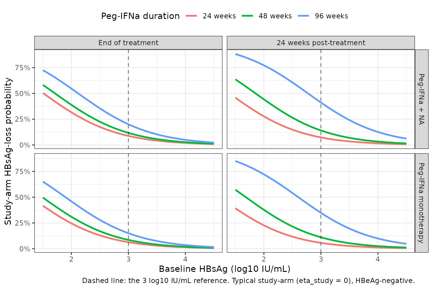
Study-arm HBsAg-loss probability against baseline HBsAg for three Peg-IFN-alpha durations, both endpoints, both regimens (typical study-arm, HBeAg-negative).
The duration effect is visibly larger at 24 weeks post-treatment than at end of treatment, which is the Table 2 result that the per-week odds ratio rises from 1.013 to 1.031.
Validation strategy: why there is no PKNCA section
The standard popPK validation for this library is a PKNCA non-compartmental analysis against the paper’s reported Cmax / AUC / half-life. That is not applicable here and is deliberately omitted:
- There is no pharmacokinetic component. Neither model contains a concentration, a dose amount, a volume or a clearance – the Peg-IFN-alpha regimen enters only as a binary combination indicator and a planned-duration covariate, because non-standard Peg-IFN-alpha dosing was an exclusion criterion.
- The model output
Ccis a dimensionless proportion in [0, 1], not a concentration. It is namedCconly to satisfy the library’s endpoint convention. - There is no time axis to integrate over: both models are cross-sectional.
The validation above substitutes the checks that can actually catch a translation error in this model class: exact reproduction of every published parameter back-transform (Check 1), odds ratios recovered from the solved model rather than from the inputs (Check 2), reconstruction of the published prediction intervals that discriminates a variance from a standard deviation (Check 3), the paper’s own simulation answer key (Check 4), the variance- reduction arithmetic (Check 5), and an internal-consistency back-solve of the answer key against the parameter table (Check 6).
Assumptions and deviations
-
Two model files, one vignette. The paper fits its
endpoints independently (Section 2.3) on different analysis sets with
different retained covariates, so the author structure is replicated as
two
.Rfiles sharing this vignette. -
addSd <- fixed(0.001)is not a paper parameter. Section 2.3.1 fixes the residual variance to 1 with a binomial variance function, so there is no estimated residual-error term. The placeholder exists only so the model declares an nlmixr2 endpoint; it is negligible and the paper’s own Table 3 simulations exclude any residual term (Section 2.5 resamples fixed effects and the study eta only). -
eta_studyis a paper-specific eta name. It is a between-study-strata-arm effect, not a between-subject effect on a structural PK parameter, so it is declared inpaper_specific_etasrather than renamed to anetal<param>form. - Simulation scope is the study arm. Every output here is an aggregate study-arm proportion. These models must not be used for individual-patient simulation.
-
HBeAg mixture handling. For an arm containing both
HBeAg strata, simulate the strata separately and take the HBeAg-weighted
average, as Check 4 does. Evaluating the model at a fractional
HBEAG_POSis wrong because the model is logit-linear in the indicator. -
Screened-but-not-retained covariates carry no
estimates. Age, gender, race, study design, and (24-week model
only) continuation of NA after Peg-IFN-alpha cessation were tested and
not retained; the paper reports no point estimate for any of them. They
are documented in
covariatesDataExcludedin each model file rather than encoded. -
Race orientation. The paper’s race covariate is the
proportion non-Asian; the register’s canonical
RACE_ASIAN_PCTis the complement. This matters only if someone revives the screened covariate, since it is not in either final model. - Base models are not extracted. The base models (single overall treatment effect, EOT 6.7% [95% PI 0.9-36.7] and 24-week 6.7% [95% PI 0.3-63.7]) are reported only through those rates and their between-trial variances; their intercepts are not tabulated, so they are not reproducible and only the final covariate models are extracted.
Errata
Discrepancies found in the source while verifying. None changes an encoded parameter value; each is recorded so a reader comparing the model file against the paper is not surprised.
-
HBeAg p-value. Table 2 prints
p = 0.008for the EOT HBeAg-status term; the Abstract and Results Section 3.3 both sayp = 0.007. Estimates are unaffected. - Between-trial variance reduction. Results Section 3.3 gives 56.5% (EOT) and 77.5% (24-week), which Check 5 confirms is the arithmetically correct pair. The Abstract and Discussion instead give 58.1% and 77.6%. The Results figures are the right ones; note this is the reverse of the usual pattern, in which the Results narrative is the one that drifts.
- Table 3, Peg-IFN-alpha + NA “<= 5 log10” row is internally inconsistent. Check 6 back-solves its published 24-week rate of 6.8% through the paper’s own Table 2 coefficients and recovers a baseline of 3.51 log10 IU/mL against a printed 3.3. Every other row back-solves to within 0.019. Either the baseline or the rate in that one row is mis-transcribed and the paper gives no way to tell which, so the row is excluded from the Check 4 and Check 6 assertions and is flagged in both tables.
- Table 2 cosmetic slips. The 24-week “Drug effect (Peg-IFNa + NA)” Interpretation cell has a doubled percent sign (“14.1% %”) and names the regimen “48 weeks Peg-IFNa” without the “+ NA”.
-
Section 3.5 rates are not reproducible from Table
2. The in-silico-trial benchmarks (15.1% monotherapy, 19.1%
combination, for virtual cohorts calibrated at baseline HBsAg 2485 and
2081 IU/mL) cannot be recovered from the Table 2 coefficients at any
plausible duration or HBeAg mix; at 2485 IU/mL = 3.40 log10 and 48 weeks
the models give roughly 4.8% (EOT) and 6.3% (24-week). Those figures
come from the companion Cortes-Rios 2025 in-silico-trial calibration
rather than from this paper’s own models, so they are not used as a
validation target. Note also that Section 3.5 is where the paper quotes
baselines in raw IU/mL while the models take
log10 IU/mL – the reason the canonical covariate is
named
HBSAG_BL_LOG10.