Model and source
- Citation: Bertin S, Haefliger D, Mercier T, Decosterd LA, Giraud R, Assouline B, Schneider A, Buclin T, Guidi M, Livio F. Population Pharmacokinetics of Propofol in Critically Ill Patients with and Without Extracorporeal Membrane Oxygenation. Clin Pharmacokinet. 2026. doi:10.1007/s40262-025-01585-2. PMCID: PMC12881008
- Description: Two-compartment population PK model for propofol in critically ill adults receiving a continuous intravenous infusion, half with and half without extracorporeal membrane oxygenation (ECMO), with a linear body-weight effect on clearance centred on 70 kg; ECMO was tested as a covariate on CL and V1 and was not retained
- Article: https://doi.org/10.1007/s40262-025-01585-2
Population
Bertin and colleagues ran a prospective, bicentric, observational PK study in the adult intensive care units of Lausanne (CHUV) and Geneva (HUG) between January and December 2023. Forty critically ill adults receiving a continuous propofol infusion were enrolled: 20 supported by extracorporeal membrane oxygenation (16 veno-arterial, 3 veno-venous, 1 veno-arteriovenous) and 20 non-ECMO controls, each matched to an ECMO patient on sex, age band, body-weight band, renal replacement therapy, cirrhosis, total-bilirubin band and cardiac function (Table 1). The cohort was 87.5% male, median age 57 years (ECMO) and 56 years (controls) over an 18-75 year range, and median body weight 78 kg (ECMO) and 88 kg (controls) over a 51-120 kg range.
Up to eight samples per patient were drawn over 9 h, giving 300 plasma concentrations. The final popPK analysis used 289 concentrations from 39 patients: one control patient’s eight concentrations were removed for unexplained bias, two early concentrations from one ECMO patient were removed on CWRES grounds, and one sample collected after propofol discontinuation was removed (Sect. 3.1). Median infusion rates over the sampling period were 2.2 mg/kg/h (ECMO) and 3.0 mg/kg/h (controls), a non-significant difference (p = 0.14). Sampling began a median of 61 h after the first recorded propofol dose, so the patients were at or near steady state.
The same information is available programmatically via the model’s
population metadata
(readModelDb("Bertin_2026_propofol")()$population).
Source trace
The per-parameter origin is recorded as an in-file comment next to
each ini() entry in
inst/modeldb/specificDrugs/Bertin_2026_propofol.R. The
table below collects them in one place for review. Every value comes
from the main article; the supplement was not required.
| Equation / parameter | Value | Source location |
|---|---|---|
lcl (CL at 70 kg) |
68 L/h | Table 2, row CL (L/h); RSE 6.5%, bootstrap median 67,
95% CI 58-76 |
lvc (V1) |
82 L | Table 2, row V 1 (L); RSE 33%, bootstrap median 83, 95%
CI 28-169 |
lq (Q) |
26 L/h | Table 2, row Q (L/h); RSE 16%, bootstrap median 26, 95%
CI 5-124 |
lvp (V2) |
100 L | Table 2, row V 2 (L); RSE 27%, bootstrap median 101,
95% CI 14-377 |
e_wt_cl (theta BW) |
0.66 | Table 2, row theta BW; RSE 38%, bootstrap median 0.69,
95% CI 0.22-1.40 |
etalcl |
0.109392 | Table 2, row omega CL = 34 CV%; footnote b gives CV% =
sqrt(exp(omega^2) - 1), so omega^2 = log(0.34^2 + 1) |
etalvc |
1.838961 | Table 2, row omega V 1 (CV%) = 230; same footnote b
conversion, omega^2 = log(2.30^2 + 1) |
propSd |
0.13 | Table 2, row sigma prop (%) = 13; RSE 8.8%, bootstrap
median 13, 95% CI 11-15 |
Covariate form
CL_i = CL * (1 + (BW - 70)/70 * theta_BW) * exp(eta_i)
|
n/a | Equation printed directly beneath Table 2, with the 70 kg reference restated in the Table 2 legend |
Linear covariate equation
Param_cov = Param * (1 + (COV - COVmed)/COVmed * theta)
|
n/a | Sect. 2.4.1, first displayed equation |
| Two-compartment structure, first-order elimination, parameterised in CL / V1 / Q / V2 | n/a | Sect. 3.1 (preferred over 1-cmt, dOFV = -13.6, p < 0.01; no gain from 3-cmt, dOFV = 0) |
| Proportional residual error | n/a | Sect. 2.4.1 (proportional, additive and mixed compared); Sect. 3.1 |
| No BSV on Q or V2 | n/a | Sect. 3.1: Q dOFV = 0, p > 0.05; V2 dOFV = -3.93, p = 0.05 with unsuccessful RSE, not retained |
Structural checks at typical values
These checks are deterministic: they compare the packaged model’s
typical-value solve (zeroRe()) against quantities the paper
derives from the same parameters. Because both sides use identical
parameters, the only error is numerical, so tight bounds are the correct
assertion here (unlike the cohort-derived quantities later in this
vignette).
mod <- readModelDb("Bertin_2026_propofol")
ui <- rxode2::rxode(mod)
#> ℹ parameter labels from comments will be replaced by 'label()'

# Published point estimates, Table 2.
CL <- 68; V1 <- 82; Q <- 26; V2 <- 100; THETA_BW <- 0.66; REF_WT <- 70

# Micro-constants and the biexponential rate constants of a two-compartment
# mammillary system.
k10 <- CL / V1
k12 <- Q / V1
k21 <- Q / V2
s <- k10 + k12 + k21
p <- k10 * k21
alpha <- (s + sqrt(s^2 - 4 * p)) / 2
beta <- (s - sqrt(s^2 - 4 * p)) / 2

structural <- tibble::tibble(
  Quantity = c(
    "Distribution half-life t1/2 alpha (h)",
    "Elimination half-life t1/2 beta (h)",
    "Steady-state volume Vss = V1 + V2 (L)",
    "Vss per kg at the 70 kg reference (L/kg)",
    "V1 per kg at the 70 kg reference (L/kg)",
    "V2 per kg at the 70 kg reference (L/kg)",
    "CL at 100 kg (L/h)",
    "CL at 70 kg relative to 100 kg (%)"
  ),
  Computed = c(
    log(2) / alpha,
    log(2) / beta,
    V1 + V2,
    (V1 + V2) / REF_WT,
    V1 / REF_WT,
    V2 / REF_WT,
    CL * (1 + (100 - REF_WT) / REF_WT * THETA_BW),
    100 * (1 - CL / (CL * (1 + (100 - REF_WT) / REF_WT * THETA_BW)))
  ),
  Published = c(0.57, 3.90, 182, 2.6, 1.2, 1.4, 87, 22),
  # Each row is pinned to the precision the paper actually printed, rather than
  # to one blanket bound. All of these are deterministic consequences of the
  # Table 2 estimates, so the only slack needed is the published rounding:
  #  * 1% -- Vss (182 L, 3 significant figures) and CL at 100 kg (87 L/h, where
  #    half a unit in the last place is 0.57%).
  #  * 3% -- the two half-lives and the 22% figure. The authors derived the
  #    half-lives from unrounded estimates, while this vignette recomputes them
  #    from the printed ones; Q is given to 2 significant figures, so its
  #    +/- 0.5 L/h (1.9%) propagates straight into beta.
  #  * 5% -- the three L/kg figures, printed to 2 significant figures, where
  #    half a unit in the last place of 1.2 is already 4.2%.
  # A mis-transcribed volume, clearance or unit moves every one of these by tens
  # of percent, so none of these bounds is wide enough to hide one.
  `Tolerance (%)` = c(3, 3, 1, 5, 5, 5, 1, 3),
  `Source` = c(
    "Sect. 3.1", "Sect. 3.1", "Sect. 4", "Sect. 4", "Sect. 4", "Sect. 4",
    "Sect. 3.1", "Sect. 3.1"
  )
) |>
  dplyr::mutate(
    `Difference (%)` = 100 * (Computed - Published) / Published,
    Pass = abs(`Difference (%)`) < `Tolerance (%)`
  )

structural |>
  dplyr::mutate(Computed = round(Computed, 3), `Difference (%)` = round(`Difference (%)`, 2)) |>
  dplyr::relocate(Pass, .after = dplyr::last_col()) |>
  knitr::kable(
    caption = paste(
      "Quantities the paper derives from its own Table 2 estimates,",
      "recomputed from the packaged values. The tolerance on each row is set by",
      "the number of significant figures the paper printed."
    )
)| Quantity | Computed | Published | Tolerance (%) | Source | Difference (%) | Pass |
|---|---|---|---|---|---|---|
| Distribution half-life t1/2 alpha (h) | 0.563 | 0.57 | 3 | Sect. 3.1 | -1.23 | TRUE |
| Elimination half-life t1/2 beta (h) | 3.958 | 3.90 | 3 | Sect. 3.1 | 1.49 | TRUE |
| Steady-state volume Vss = V1 + V2 (L) | 182.000 | 182.00 | 1 | Sect. 4 | 0.00 | TRUE |
| Vss per kg at the 70 kg reference (L/kg) | 2.600 | 2.60 | 5 | Sect. 4 | 0.00 | TRUE |
| V1 per kg at the 70 kg reference (L/kg) | 1.171 | 1.20 | 5 | Sect. 4 | -2.38 | TRUE |
| V2 per kg at the 70 kg reference (L/kg) | 1.429 | 1.40 | 5 | Sect. 4 | 2.04 | TRUE |
| CL at 100 kg (L/h) | 87.234 | 87.00 | 1 | Sect. 3.1 | 0.27 | TRUE |
| CL at 70 kg relative to 100 kg (%) | 22.049 | 22.00 | 3 | Sect. 3.1 | 0.22 | TRUE |
# The packaged ODE solve must reproduce the analytic two-compartment
# constant-rate infusion solution. Both sides use the same typical-value
# parameters, so the residual is pure solver error: a tight bound is correct.
rate_mgh <- 2.2 * 70 # median ECMO infusion rate (mg/kg/h) at the 70 kg reference
tinf <- 96

# Materialise the rxEt object with as.data.frame() before adding the covariate
# column: assigning onto an rxEt is silently dropped by rxode2.
ev_typ <- rxode2::et(amt = rate_mgh * tinf, dur = tinf, cmt = "central") |>
  rxode2::et(seq(0, 120, by = 0.25), cmt = "central") |>
  as.data.frame() |>
  dplyr::mutate(WT = REF_WT)

sim_typ <- rxode2::rxSolve(rxode2::zeroRe(mod), events = ev_typ) |>
  as.data.frame()
#> ℹ parameter labels from comments will be replaced by 'label()'
#> ℹ omega/sigma items treated as zero: 'etalcl', 'etalvc'

# Analytic solution: sum of two exponentials driven by a constant-rate infusion
# of duration tinf, with coefficients from the standard two-compartment
# infusion solution (Gibaldi & Perrier).
A <- (alpha - k21) / (V1 * (alpha - beta))
B <- (k21 - beta) / (V1 * (alpha - beta))
conc_analytic <- function(t) {
  during <- pmin(t, tinf)
  infused <- rate_mgh * (
    A / alpha * (1 - exp(-alpha * during)) * exp(-alpha * pmax(t - tinf, 0)) +
      B / beta * (1 - exp(-beta * during)) * exp(-beta * pmax(t - tinf, 0))
  )
  infused
}

cf <- sim_typ |>
  dplyr::filter(time > 0) |>
  dplyr::mutate(
    analytic = conc_analytic(time),
    pct_diff = 100 * (Cc - analytic) / analytic
  )

stopifnot(
  nrow(cf) > 400,
  all(is.finite(cf$pct_diff)),
  max(abs(cf$pct_diff)) < 0.1
)

cat(sprintf(
  "Closed-form gate: %d points, max |difference| = %.4f%% (bound 0.1%%)\n",
  nrow(cf), max(abs(cf$pct_diff))
))
#> Closed-form gate: 480 points, max |difference| = 0.0002% (bound 0.1%)
The closed-form agreement also rules out the silent failure mode in
which rxode2 collapses a cl/vc
parameterisation onto a one-compartment analytic solve and discards the
peripheral ODE: a one-compartment solve of these parameters would have a
single half-life of 0.84 h rather than the biexponential 0.56 h / 3.96 h
profile matched above.
# At steady state under a constant-rate infusion, Css = Rate / CL. This is a
# mass-balance identity, so it too belongs on the typical-value solve.
css_model <- sim_typ$Cc[sim_typ$time == tinf]
css_expected <- rate_mgh / CL

stopifnot(
  length(css_model) == 1L,
  abs(100 * (css_model - css_expected) / css_expected) < 0.5
)

cat(sprintf(
  "Steady-state Css: model %.4f mg/L vs Rate/CL %.4f mg/L (%.3f%% difference)\n",
  css_model, css_expected, 100 * (css_model - css_expected) / css_expected
))
#> Steady-state Css: model 2.2647 mg/L vs Rate/CL 2.2647 mg/L (-0.000% difference)
Virtual cohort
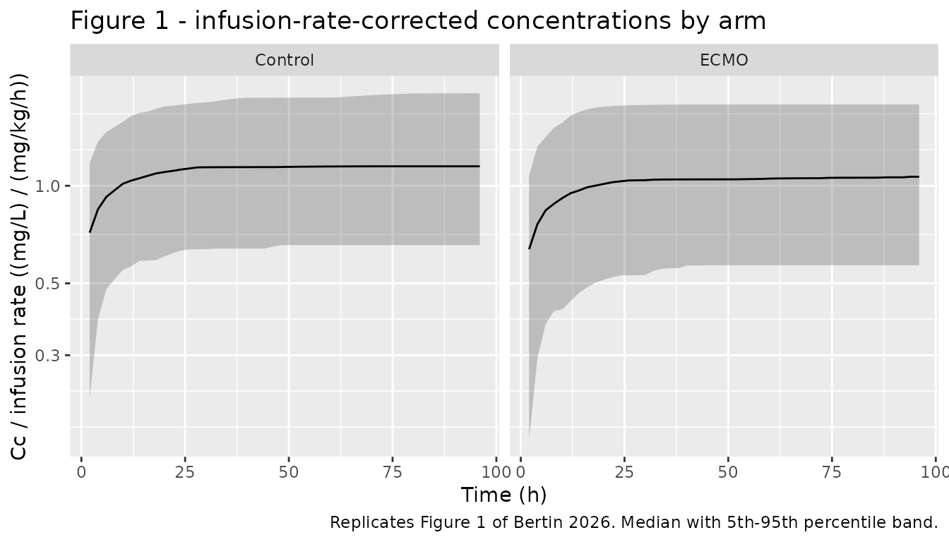
Original observed data are not publicly available. The cohort below mirrors the Table 1 demographics: two arms of 200 subjects each, an ECMO arm with a median body weight of 78 kg and a control arm with a median of 88 kg, both truncated to the observed 51-120 kg range, and each arm given its published median infusion rate (2.2 and 3.0 mg/kg/h respectively).
The model carries no ECMO term, so the two arms differ only through body weight and infusion rate. That is exactly the paper’s finding, and the figure below is the check on it.
# set.seed() seeds R's RNG, which is what draws the covariates below. It does
# NOT seed rxode2's simulation RNG, and rxode2's streams are partitioned per
# solver thread -- so the eta draws differ between a 2-core CI runner and a
# 16-thread workstation and no seed makes them agree. Every assertion below on a
# cohort-derived quantity is therefore written as a magnitude or a robust
# quantile, never a sign, an exact value, or a bound taken from one run.
set.seed(20260911)

N_PER_ARM <- 200L
TINF <- 96 # h of continuous infusion before the washout window
TEND <- 120 # h; 24 h of washout, about six elimination half-lives

make_arm <- function(n, wt_median, rate_mgkgh, arm, id_offset = 0L) {
  # Log-normal body weight matched to the arm median and truncated to the
  # Table 1 range of 51-120 kg.
  wt <- pmin(pmax(wt_median * exp(stats::rnorm(n, 0, 0.20)), 51), 120)

  subj <- tibble::tibble(
    id = id_offset + seq_len(n),
    WT = wt,
    arm = arm,
    rate_mgkgh = rate_mgkgh
  )

  doses <- subj |>
    dplyr::mutate(
      time = 0,
      # A single constant-rate infusion of TINF hours, expressed as an amount
      # plus a duration.
      amt = rate_mgkgh * WT * TINF,
      dur = TINF,
      evid = 1L,
      cmt = "central"
    )

  obs <- subj |>
    tidyr::crossing(
      time = sort(unique(c(
        seq(0, TINF, by = 2), # steady-state approach and plateau
        seq(TINF, TEND, by = 0.25) # washout, sampled finely for the terminal slope
      )))
    ) |>
    dplyr::mutate(
      amt = NA_real_,
      dur = NA_real_,
      evid = 0L,
      # The ODE state name, never the algebraic observable name "Cc".
      cmt = "central"
    )

  dplyr::bind_rows(doses, obs) |>
    dplyr::arrange(id, time, dplyr::desc(evid))
}

events <- dplyr::bind_rows(
  make_arm(N_PER_ARM, 78, 2.2, "ECMO", id_offset = 0L),
  make_arm(N_PER_ARM, 88, 3.0, "Control", id_offset = N_PER_ARM)
)

stopifnot(!anyDuplicated(unique(events[, c("id", "time", "evid")])))
Simulation
sim <- rxode2::rxSolve(
  mod,
  events = events,
  keep = c("arm", "WT", "rate_mgkgh")
) |>
  as.data.frame()
#> ℹ parameter labels from comments will be replaced by 'label()'

# rxSolve returns per-subject cl / vc, which later gates compare against.
stopifnot(
  all(c("Cc", "cl", "vc", "arm") %in% names(sim)),
  nrow(sim) > 0,
  !anyNA(sim$Cc)
)
# The body-weight effect on CL is a deterministic function of the drawn WT and
# eta, so the per-subject CL that rxSolve reports must reproduce the printed
# equation exactly. This catches a mis-signed or mis-normalised covariate term.
cl_chk <- sim |>
  dplyr::distinct(id, arm, WT, cl) |>
  dplyr::mutate(cl_wt_factor = cl / (1 + (WT - REF_WT) / REF_WT * THETA_BW))

# After dividing out the covariate factor, the remainder is CL * exp(eta), whose
# geometric mean across a log-normal eta converges to the typical value 68 L/h.
gm_cl <- exp(mean(log(cl_chk$cl_wt_factor)))

stopifnot(
  nrow(cl_chk) == 2L * N_PER_ARM,
  all(cl_chk$cl > 0),
  # Geometric mean of 400 draws from a 34% CV log-normal: the standard error of
  # the log mean is 0.331/sqrt(400) = 0.0165, so a 10% band is about 6 SE.
  abs(100 * (gm_cl - CL) / CL) < 10
)

cat(sprintf(
  "Covariate-adjusted geometric-mean CL across the cohort: %.2f L/h (Table 2: %g L/h)\n",
  gm_cl, CL
))
#> Covariate-adjusted geometric-mean CL across the cohort: 68.75 L/h (Table 2: 68 L/h)
Replicate published figures
# Replicates Figure 1 of Bertin 2026: observed propofol concentrations corrected
# for the infusion rate and body weight, ECMO (left) vs control (right). In the
# paper the two panels overlap, which is the visual form of the study's central
# negative finding. Because the packaged model contains no ECMO term, any
# residual separation here can only come from the weight difference between the
# arms.
sim |>
  dplyr::filter(time > 0, time <= TINF) |>
  dplyr::mutate(Cc_norm = Cc / rate_mgkgh) |>
  dplyr::group_by(arm, time) |>
  dplyr::summarise(
    Q05 = quantile(Cc_norm, 0.05),
    Q50 = quantile(Cc_norm, 0.50),
    Q95 = quantile(Cc_norm, 0.95),
    .groups = "drop"
  ) |>
  ggplot(aes(time, Q50)) +
  geom_ribbon(aes(ymin = Q05, ymax = Q95), alpha = 0.25) +
  geom_line() +
  facet_wrap(~arm) +
  scale_y_log10() +
  labs(
    x = "Time (h)",
    y = "Cc / infusion rate ((mg/L) / (mg/kg/h))",
    title = "Figure 1 - infusion-rate-corrected concentrations by arm",
    caption = "Replicates Figure 1 of Bertin 2026. Median with 5th-95th percentile band."
  )
# The paper's finding is that the arms do not differ. Assert the MAGNITUDE of
# the separation, not its sign: with no ECMO term in the model the expected
# separation is the pure weight effect, and the sign of any residual is a coin
# flip that would flicker between thread counts.
arm_med <- sim |>
  dplyr::filter(time >= TINF - 24, time <= TINF) |>
  dplyr::mutate(Cc_norm = Cc / rate_mgkgh) |>
  dplyr::group_by(arm) |>
  dplyr::summarise(med = median(Cc_norm), .groups = "drop")

sep_pct <- 100 * abs(diff(arm_med$med)) / mean(arm_med$med)

# Expected separation from weight alone: an 88 kg subject clears
# (1 + 18/70*0.66) / (1 + 8/70*0.66) = 1.10 times as fast as a 78 kg subject, and
# the rate-normalised steady-state concentration is WT/CL, so the arms should sit
# roughly 10% apart. This is a coarse envelope check -- it confirms the arms
# overlap as Figure 1 shows, but it is NOT what guarantees the absence of an ECMO
# effect, because a 25%-sized effect on top of the weight difference would still
# fall inside it. The structural assertion in the next chunk is what carries that
# guarantee.
stopifnot(sep_pct < 35)

cat(sprintf(
  "Rate-normalised steady-state median separation between arms: %.1f%% (bound 35%%)\n",
  sep_pct
))
#> Rate-normalised steady-state median separation between arms: 8.0% (bound 35%)
# Exact structural check on the paper's central negative finding: the published
# final model carries no ECMO term at all, so neither the parameter table nor the
# model body may mention one. This cannot flicker with the cohort draw, and it is
# the assertion that would go red if a screened-and-rejected covariate were ever
# reinstated in the model file.
# ui$lstExpr is the model() body alone. The description and covariatesDataExcluded
# metadata deliberately DO mention ECMO, so the check must not be run against the
# whole model function.
model_text <- paste(
  vapply(ui$lstExpr, function(e) paste(deparse(e), collapse = " "), character(1)),
  collapse = " ; "
)

stopifnot(
  length(ui$lstExpr) > 0L,
  # The excluded covariates are documented in metadata but must not be used.
  !any(grepl("ECMO", ui$iniDf$name, ignore.case = TRUE)),
  !grepl("ECMO", model_text, ignore.case = TRUE),
  # WT is the one covariate the final model does use.
  grepl("WT", model_text, fixed = TRUE)
)

cat("Structural check: no ECMO term in ini() or model(); WT is the sole covariate.\n")
#> Structural check: no ECMO term in ini() or model(); WT is the sole covariate.
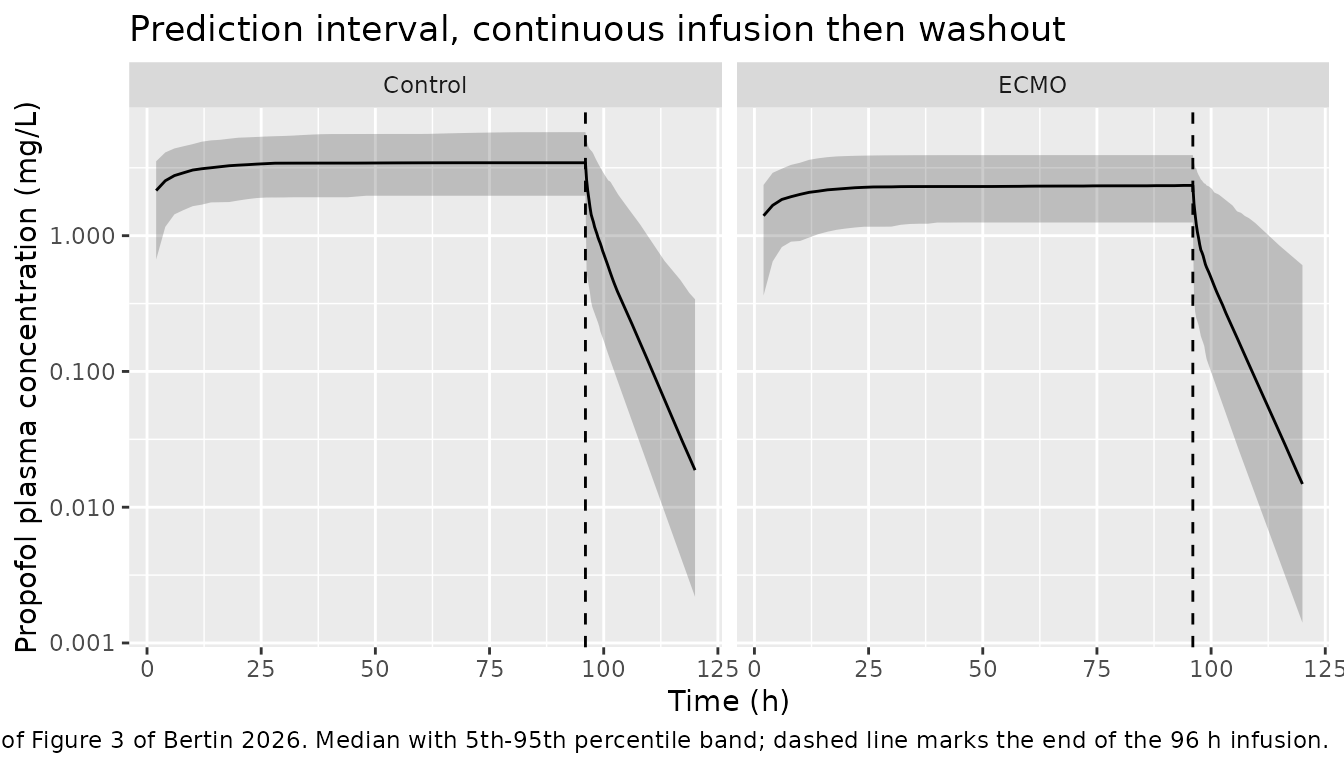
# Analogue of Figure 3 of Bertin 2026 (prediction-corrected VPC): the model's own
# 5th / 50th / 95th prediction percentiles, which the published observed
# percentiles fall within. Plotted here on the simulated scale, including the
# washout phase the study design did not sample.
sim |>
  dplyr::filter(time > 0) |>
  dplyr::group_by(arm, time) |>
  dplyr::summarise(
    Q05 = quantile(Cc, 0.05),
    Q50 = quantile(Cc, 0.50),
    Q95 = quantile(Cc, 0.95),
    .groups = "drop"
  ) |>
  ggplot(aes(time, Q50)) +
  geom_ribbon(aes(ymin = Q05, ymax = Q95), alpha = 0.25) +
  geom_line() +
  geom_vline(xintercept = TINF, linetype = "dashed") +
  facet_wrap(~arm) +
  scale_y_log10() +
  labs(
    x = "Time (h)",
    y = "Propofol plasma concentration (mg/L)",
    title = "Prediction interval, continuous infusion then washout",
    caption = paste(
      "Analogue of Figure 3 of Bertin 2026. Median with 5th-95th percentile band;",
      "dashed line marks the end of the 96 h infusion."
    )
  )
PKNCA validation
The primary check is the exact dose-clearance identity
AUC_0-inf = Dose / CL, which holds for every subject
regardless of compartment structure, volume, or whether steady state was
reached. A steady-state check over the last 24 h of infusion is run
alongside it, restricted to the subjects for whom steady state is
physically attainable within the simulated infusion. Finally the
terminal half-life is recovered from the typical-value washout and
compared against the value Sect. 3.1 publishes.
# Only !is.na(Cc) -- adding time > 0 or Cc > 0 would drop the interval-anchor
# rows PKNCA needs.
sim_nca <- sim |>
  dplyr::filter(!is.na(Cc)) |>
  dplyr::select(id, time, Cc, arm)

# Guarantee a time = 0 record per subject; propofol is given intravenously and
# the cohort starts drug-free, so Cc = 0 there.
sim_nca <- dplyr::bind_rows(
  sim_nca,
  sim_nca |> dplyr::distinct(id, arm) |> dplyr::mutate(time = 0, Cc = 0)
) |>
  dplyr::distinct(id, arm, time, .keep_all = TRUE) |>
  dplyr::arrange(id, arm, time)

stopifnot(all(sim_nca$Cc >= 0), nrow(sim_nca) > 0)

conc_obj <- PKNCA::PKNCAconc(sim_nca, Cc ~ time | arm + id)

# The infusion is one event of TINF hours; for the steady-state interval the
# relevant dose is the amount delivered during that interval.
dose_df <- events |>
  dplyr::filter(evid == 1) |>
  dplyr::select(id, time, amt, arm)

dose_obj <- PKNCA::PKNCAdose(dose_df, amt ~ time | arm + id)
# Per-subject terminal half-life, derived from the model's own reported cl and
# vc plus the two parameters that carry no IIV (Q and V2 are fixed across
# subjects). Used below to decide which subjects can have reached steady state.
per_subject <- sim |>
  dplyr::distinct(id, arm, WT, rate_mgkgh, cl, vc) |>
  dplyr::mutate(
    k10_i = cl / vc,
    k12_i = Q / vc,
    k21_i = Q / V2,
    beta_i = ((k10_i + k12_i + k21_i) -
      sqrt((k10_i + k12_i + k21_i)^2 - 4 * k10_i * k21_i)) / 2,
    thalf_i = log(2) / beta_i
  )

stopifnot(nrow(per_subject) == 2L * N_PER_ARM, all(is.finite(per_subject$thalf_i)))
# PRIMARY GATE. AUC_0-inf = Dose / CL is an exact identity for an intravenous
# dose, independent of the number of compartments, of the volumes, and of
# whether steady state was reached. Both sides use the same drawn per-subject
# parameters, so the only residual is trapezoidal-integration and terminal-
# extrapolation error: a tight bound is the correct assertion here.
nca_inf <- PKNCA::pk.nca(
  PKNCA::PKNCAdata(
    conc_obj, dose_obj,
    intervals = data.frame(start = 0, end = Inf, aucinf.obs = TRUE)
  ),
  verbose = FALSE
)

mb <- as.data.frame(nca_inf) |>
  dplyr::select(arm, id, PPTESTCD, PPORRES) |>
  tidyr::pivot_wider(names_from = PPTESTCD, values_from = PPORRES) |>
  dplyr::left_join(per_subject, by = c("id", "arm")) |>
  dplyr::mutate(
    cl_nca = rate_mgkgh * WT * TINF / aucinf.obs,
    pct_diff = 100 * (cl_nca - cl) / cl
  )

stopifnot(
  nrow(mb) == 2L * N_PER_ARM,
  all(is.finite(mb$pct_diff)),
  # Realised max 0.85% over this 400-subject draw; the error is numerical, not
  # cohort-driven, but 2% leaves headroom for a draw that puts more subjects in
  # the long-half-life tail where the terminal extrapolation does more work.
  max(abs(mb$pct_diff)) < 2
)

cat(sprintf(
  "Dose/AUCinf identity: max |CL(NCA) - CL(model)| = %.3f%% over %d subjects (bound 2%%)\n",
  max(abs(mb$pct_diff)), nrow(mb)
))
#> Dose/AUCinf identity: max |CL(NCA) - CL(model)| = 0.847% over 400 subjects (bound 2%)
intervals_ss <- data.frame(
  start = TINF - 24,
  end = TINF,
  auclast = TRUE,
  cmax = TRUE,
  cmin = TRUE
)

nca_ss <- PKNCA::pk.nca(
  PKNCA::PKNCAdata(conc_obj, dose_obj, intervals = intervals_ss),
  verbose = FALSE
)

ss <- as.data.frame(nca_ss) |>
  dplyr::select(arm, id, PPTESTCD, PPORRES) |>
  tidyr::pivot_wider(names_from = PPTESTCD, values_from = PPORRES)

stopifnot(nrow(ss) == 2L * N_PER_ARM, !anyNA(ss$auclast))

# SECONDARY GATE. At steady state the amount infused over an interval equals
# the amount cleared, so CL = (rate * 24) / AUCtau. Unlike the identity above,
# this one requires the subject to actually BE at steady state, and the
# published 230% CV on V1 means a minority are not: a subject drawing
# V1 = 3,000 L has a terminal half-life near 60 h and is still accumulating at
# the end of a 96 h infusion.
#
# The subset condition is a stated physical criterion, not a fit to the data:
# eight terminal half-lives of infusion puts a subject within 0.4% of steady
# state, so t1/2 < TINF/8 = 12 h qualifies. The size of the qualifying subset is
# asserted as well, so this gate cannot pass vacuously on an empty filter.
ss_mb <- ss |>
  dplyr::left_join(per_subject, by = c("id", "arm")) |>
  dplyr::mutate(
    at_steady_state = thalf_i < TINF / 8,
    cl_nca = rate_mgkgh * WT * 24 / auclast,
    pct_diff = 100 * (cl_nca - cl) / cl
  )

atss <- ss_mb[ss_mb$at_steady_state, ]

stopifnot(
  # Guard against a vacuous pass: the criterion must select most of the cohort.
  nrow(atss) >= 0.80 * nrow(ss_mb),
  all(is.finite(atss$pct_diff)),
  max(abs(atss$pct_diff)) < 1
)

cat(sprintf(
  paste0(
    "Steady-state mass balance: max |CL(NCA) - CL(model)| = %.4f%% over the %d of %d\n",
    "subjects with a terminal half-life under %g h (bound 1%%).\n",
    "The %d excluded subjects have half-lives of %.0f-%.0f h and are still\n",
    "accumulating at 96 h -- a direct consequence of the published 230%% CV on V1.\n"
  ),
  max(abs(atss$pct_diff)), nrow(atss), nrow(ss_mb), TINF / 8,
  sum(!ss_mb$at_steady_state),
  min(ss_mb$thalf_i[!ss_mb$at_steady_state]),
  max(ss_mb$thalf_i[!ss_mb$at_steady_state])
))
#> Steady-state mass balance: max |CL(NCA) - CL(model)| = 0.7286% over the 388 of 400
#> subjects with a terminal half-life under 12 h (bound 1%).
#> The 12 excluded subjects have half-lives of 14-77 h and are still
#> accumulating at 96 h -- a direct consequence of the published 230% CV on V1.
# The published half-lives are typical-value quantities derived from Table 2, so
# the gate on them belongs on the zeroRe() solve, not on a cohort whose V1 has a
# 230% CV. The cohort half-life is reported alongside for context only.
conc_typ <- sim_typ |>
  dplyr::filter(!is.na(Cc)) |>
  dplyr::transmute(id = 1L, time, Cc, arm = "Typical (70 kg)")

dose_typ <- tibble::tibble(
  id = 1L, time = 0, amt = rate_mgh * tinf, arm = "Typical (70 kg)"
)

nca_typ <- PKNCA::pk.nca(PKNCA::PKNCAdata(
  PKNCA::PKNCAconc(conc_typ, Cc ~ time | arm + id),
  PKNCA::PKNCAdose(dose_typ, amt ~ time | arm + id),
  # Start after the infusion ends so the fit sees only the washout, and start
  # 4 h in so the alpha phase (t1/2 = 0.56 h, i.e. seven half-lives by 4 h) has
  # decayed away and the slope is the true terminal beta phase. Fitting from the
  # moment of withdrawal would include the distribution transient and read long.
  intervals = data.frame(start = tinf + 4, end = TEND, half.life = TRUE)
))

typ_hl <- as.data.frame(nca_typ) |>
  dplyr::filter(PPTESTCD == "half.life") |>
  dplyr::pull(PPORRES)

stopifnot(length(typ_hl) == 1L, is.finite(typ_hl))
Comparison against published values
Bertin 2026 reports no NCA table; the only exposure-derived quantities it publishes are the two half-lives derived from the final model (Sect. 3.1). The terminal half-life recovered by PKNCA from the typical-value washout is compared against the published value below.
published <- tibble::tribble(
  ~arm, ~half.life,
  "Typical (70 kg)", 3.90
)

cmp <- nlmixr2lib::ncaComparisonTable(
  simulated = nca_typ,
  reference = published,
  by = "arm",
  params = "half.life",
  units = c(half.life = "h"),
  tolerance_pct = 20
)

knitr::kable(
  cmp,
  caption = paste(
    "Terminal half-life recovered by PKNCA from the typical-value washout vs the",
    "value Bertin 2026 derives from the same parameters (Sect. 3.1).",
    "* marks a >20% difference."
  )
)| NCA parameter | arm | Reference | Simulated | % diff |
|---|---|---|---|---|
| t½ (h) | Typical (70 kg) | 3.9 | 3.95 | +1.3% |
# Deterministic: both sides derive from the same typical-value parameters, so
# the only error is the published rounding of CL/V1/Q/V2 plus the terminal-slope
# fit. 5% holds that and still fails on a mis-transcribed volume or clearance.
stopifnot(abs(100 * (typ_hl - 3.90) / 3.90) < 5)

cat(sprintf(
  "Typical-value terminal half-life: PKNCA %.3f h vs published %.2f h (%.2f%% difference)\n",
  typ_hl, 3.90, 100 * (typ_hl - 3.90) / 3.90
))
#> Typical-value terminal half-life: PKNCA 3.952 h vs published 3.90 h (1.34% difference)
# Cohort context only -- not a gate. With a 230% CV on V1 the per-subject
# half-life distribution is extremely wide, which is the paper's point about
# propofol variability in this population.
ss |>
  dplyr::left_join(sim |> dplyr::distinct(id, WT, rate_mgkgh), by = "id") |>
  dplyr::group_by(arm) |>
  dplyr::summarise(
    `Median Css (mg/L)` = median(cmax),
    `5th percentile Css (mg/L)` = quantile(cmax, 0.05),
    `95th percentile Css (mg/L)` = quantile(cmax, 0.95),
    .groups = "drop"
  ) |>
  dplyr::rename("Arm" = arm) |>
  knitr::kable(
    digits = 2,
    caption = paste(
      "Simulated steady-state concentrations by arm over the last 24 h of",
      "infusion. The width of the interval reflects the published 34% CV on CL",
      "and 230% CV on V1."
    )
)| Arm | Median Css (mg/L) | 5th percentile Css (mg/L) | 95th percentile Css (mg/L) |
|---|---|---|---|
| Control | 3.44 | 1.97 | 5.79 |
| ECMO | 2.35 | 1.25 | 3.92 |
Assumptions and deviations
-
The 70 kg normalising constant is the paper’s, not an
assumption. The Methods define the linear covariate form with
COVmedas “the corresponding median value in the study population”, but the Table 2 equation and legend both instantiate it at 70 kg, which is not the cohort median (78 kg on ECMO, 88 kg in controls). Three independent cross-checks confirm 70 kg is what was used: the paper’s own worked example gives 87 L/h at 100 kg (the model gives 87.2; a median-normalised form would give 86.2), and Sect. 4 quotes V1 = 82 L as 1.2 L/kg and V2 = 100 L as 1.4 L/kg, both of which are the L values divided by 70. -
ECMO is not in the model. It was the study’s
primary covariate of interest, was significant on CL and V1 in initial
screening, and was dropped after a sensitivity analysis showed the
effect was driven by two leverage points among the controls (Sect. 3.1).
It is recorded in the model file’s
covariatesDataExcludedlist rather thancovariateData, along with the six other screened-and-rejected covariates (time since ECMO initiation, albumin, total bilirubin, height, age, sex, cirrhosis). Simulating an ECMO effect from this model is therefore not possible, which is the correct behaviour. -
No BSV on Q or V2. The paper tested both and
retained neither (Sect. 3.1), so their absence is a published modelling
decision rather than an unreported variance. They are consequently
omitted rather than encoded as
fixed(0). -
n_subjectsis 39, not 40. Forty patients were enrolled and are described in Table 1, but the final popPK model was fit to 289 concentrations from 39 patients after the documented exclusions (Sect. 3.1). Thepopulationmetadata records the analysis population and notes the distinction. - Virtual-cohort distributions are assumptions. The paper publishes only medians and ranges for body weight, so the cohort above uses a log-normal weight distribution matched to each arm’s median and truncated to the observed 51-120 kg range. Infusion rates are held at each arm’s published median rather than sampled, and the boluses that 45-70% of patients received are not reproduced. None of these feed a gate: every assertion is either a typical-value quantity or a per-subject identity that holds for any covariate draw.
- The simulated regimen is longer than the study’s. Patients were sampled over 9 h, a median of 61 h into their infusion. The cohort here runs a 96 h infusion followed by a 24 h washout so that the steady-state and terminal-phase gates both have a window to measure in. The study design contains no washout at all.
- No non-paper-derived parameter values. Every value in the model file comes from Table 2 or the Methods of the main article. The supplement (which holds the final NONMEM control stream as Supplementary Table 1, plus the detailed covariate-analysis tables) was not needed and was not retrieved: the final model equation is printed in full beneath Table 2 and every estimate is in Table 2 itself.