Atorvastatin (Stillemans 2022)
Source:vignettes/articles/Stillemans_2022_atorvastatin.Rmd
Stillemans_2022_atorvastatin.RmdModel and source
#> ℹ parameter labels from comments will be replaced by 'label()'Citation: Stillemans G, Paquot A, Muccioli GG, Hoste E, Panin N, Asberg A, Balligand JL, Haufroid V, Elens L. Atorvastatin population pharmacokinetics in a real-life setting: Influence of genetic polymorphisms and association with clinical response. Clin Transl Sci. 2022;15(3):667-679. doi:10.1111/cts.13185.
Article: https://doi.org/10.1111/cts.13185
Description: Two-compartment population PK model with first-order absorption for atorvastatin acid in adult ambulatory patients at cardiovascular risk (Stillemans 2022), fitted jointly to a sparsely sampled real-life investigation cohort and two richly sampled support datasets. Apparent clearance CL/F carries a separate typical value and a separate log-normal random effect for the investigation cohort and for the support datasets (STUDY_ATORVA_SUPPORT); in the investigation cohort CL/F is reduced by the SLCO1B1 c.521T>C (rs4149056) genotype, CL/F = theta_CL * (1 + theta_SLCO1B1), with separate heterozygous and homozygous-variant effects. Q/F, Vc/F and Vp/F carry log-normal IIV; ka is fixed to 2.5 1/h with no IIV. Exponential residual error.
Stillemans 2022 built a two-compartment population PK model for atorvastatin acid from sparse, opportunistic samples collected in ambulatory patients during routine care, supported by two richly sampled historical datasets. The paper’s clinical question is whether the individual apparent clearance (CL/F) estimated by the model identifies patients at risk of statin-related myalgia and predicts the cholesterol-lowering response. This article packages the PopPK model; the PK/PD part of the paper is a set of univariate regressions of individual CL/F on the outcomes and is not a simulatable model (see Assumptions and deviations).
Population
Three datasets were pooled (Supplementary Table S1):
- Investigation cohort – 70 ambulatory patients with hypercholesterolemia treated with atorvastatin 5-80 mg once daily at the Cliniques Universitaires Saint-Luc, Brussels (NCT03604471), with normal hepatic function. Each patient gave one sample per visit at 1-4 visits (132 PK samples); the post-intake delay was self-reported and ranged 2.2-40 h (median 14.6 h). Median age 53.8 years (IQR 21.6), 50% female, median BMI 26.0 kg/m^2, 94.3% White, 2.9% Hispanic and 2.9% other; 91.4% primary prevention (Table 1). SLCO1B1 c.521T>C genotypes were TT 44, TC 16, CC 5 and 5 missing (Table 2).
- Lemahieu 2005 – 13 healthy volunteers, 6 h profiles on 40 mg q24h, control phase (atorvastatin alone) of a calcineurin-inhibitor interaction study.
- Hermann 2006 – 13 patients with statin-induced myopathy and 15 healthy controls, 24 h profiles on 10 mg.
Only the investigation cohort carried covariate information, which is
why the model gives CL/F one typical value and one random effect per
cohort (STUDY_ATORVA_SUPPORT).
str(readModelDb("Stillemans_2022_atorvastatin")()$population)
#> List of 12
#>  $ species                     : chr "human"
#>  $ n_subjects                  : int 111
#>  $ n_studies                   : int 3
#>  $ n_observations_investigation: int 132
#>  $ age_median                  : chr "53.8 years (IQR 21.6), investigation cohort"
#>  $ bmi_median                  : chr "26.0 kg/m^2 (IQR 5.4), investigation cohort"
#>  $ sex_female_pct              : num 50
#>  $ race_ethnicity              : Named num [1:3] 94.3 2.9 2.9
#>   ..- attr(*, "names")= chr [1:3] "White" "Hispanic" "Other"
#>  $ disease_state               : chr "Investigation cohort: ambulatory adults with hypercholesterolemia at risk of cardiovascular disease (91.4% prim"| __truncated__
#>  $ dose_range                  : chr "Oral atorvastatin 5-80 mg q24h in the investigation cohort (20 mg 31.4%, 40 mg 27.1%, 10 mg 20.0%, 80 mg 14.3%,"| __truncated__
#>  $ regions                     : chr "Belgium (investigation cohort, Cliniques Universitaires Saint-Luc, Brussels); support-dataset sites not stated in the paper"
#>  $ notes                       : chr "Three datasets (Stillemans 2022 Supplementary Table S1): investigation cohort n = 70 patients, sparse opportuni"| __truncated__
Source trace
Every ini() value carries an in-file comment in
inst/modeldb/specificDrugs/Stillemans_2022_atorvastatin.R;
they are collected here.
| Equation / parameter | Value | Source location |
|---|---|---|
lcl_invest (CL/F, investigation cohort, 521TT) |
log(535) L/h | Table 3, theta CL investigation |
lcl_support (CL/F, support datasets) |
log(400) L/h | Table 3, theta CL support |
lq (Q/F) |
log(1690) L/h | Table 3, theta Q |
lvc (Vc/F) |
log(1960) L | Table 3, theta Vc |
lvp (Vp/F) |
log(3900) L | Table 3, theta Vp |
lka (ka) |
fixed(log(2.5)) 1/h | Table 3 (fixed); Results, Structural model |
e_snp_slco1b1_rs4149056_het_cl |
-0.402 | Table 3, theta SLCO1B1 521TC |
e_snp_slco1b1_rs4149056_hom_cl |
-0.041 | Table 3, theta SLCO1B1 521CC |
etalcl_invest |
0.0677 (variance) | Results, Covariate analysis; Table 3 prints 0.068 |
etalcl_support |
0.195 (variance) | Table 3, omega CL support |
etalq |
0.715 (variance) | Table 3, omega Q |
etalvc |
1.18 (variance) | Table 3, omega Vc |
etalvp |
0.508 (variance) | Table 3, omega Vp |
expSd |
sqrt(0.085) = 0.2915 | Table 3, sigma; exponential error (Results, Structural model) |
| CL/F = theta_CL x (1 + theta_SLCO1B1) in the investigation cohort | – | Table 3 footnote |
| Split CL/F (two thetas, two etas) by cohort | – | Results, Covariate analysis |
| Two-compartment, first-order absorption | – | Methods, Structural model; Results, Structural model |
| No IIV on ka; diagonal omega | – | Results, Structural model |
Omega and sigma scale
Table 3 labels each omega and the sigma row “(SD)”, but the printed estimates are NONMEM variances. For every omega row the midpoint of the printed 95% CI equals the square root of the printed estimate, so the CI is on the SD scale and the estimate is not; for sigma the printed CI (0.067-0.103) is the variance-scale interval implied by an SD-scale RSE of 5.5%. The Results text independently gives the CL/F variance as 0.127 before and 0.0677 after the SLCO1B1 covariate was added.
omega_rows <- tibble::tribble(
  ~parameter,       ~estimate, ~ci_low, ~ci_high,
  "CL investigation", 0.0677,  0.176,   0.344,
  "CL support",       0.195,   0.357,   0.527,
  "Q",                0.715,   0.526,   1.164,
  "Vc",               1.18,    0.745,   1.435,
  "Vp",               0.508,   0.441,   0.985
) |>
  mutate(
    sqrt_estimate = sqrt(estimate),
    ci_midpoint = (ci_low + ci_high) / 2
  )
omega_rows |>
  dplyr::rename(
    "Parameter" = parameter,
    "Printed estimate" = estimate,
    "sqrt(estimate)" = sqrt_estimate,
    "95% CI midpoint" = ci_midpoint
  ) |>
  dplyr::select(-ci_low, -ci_high) |>
knitr::kable(digits = 3)| Parameter | Printed estimate | sqrt(estimate) | 95% CI midpoint |
|---|---|---|---|
| CL investigation | 0.068 | 0.260 | 0.260 |
| CL support | 0.195 | 0.442 | 0.442 |
| Q | 0.715 | 0.846 | 0.845 |
| Vc | 1.180 | 1.086 | 1.090 |
| Vp | 0.508 | 0.713 | 0.713 |
# Deterministic arithmetic on printed numbers: sqrt(estimate) reproduces the
# CI midpoint to the table's rounding.
stopifnot(all(abs(omega_rows$sqrt_estimate - omega_rows$ci_midpoint) < 0.005))

# Sigma: SD-scale RSE 5.5% -> variance-scale RSE 11%; 95% CI on the variance.
sigma_ci <- 0.085 + c(-1, 1) * qnorm(0.975) * 0.085 * 2 * 0.055
stopifnot(all(abs(sigma_ci - c(0.067, 0.103)) < 0.002))
Typical-value profiles
Steady-state profiles over one 24 h dosing interval of 40 mg q24h for the typical patient of each investigation-cohort SLCO1B1 c.521T>C genotype and for the typical support-dataset subject.
mod <- readModelDb("Stillemans_2022_atorvastatin")
mod_typ <- rxode2::zeroRe(mod)
#> ℹ parameter labels from comments will be replaced by 'label()'

typ_groups <- tibble::tribble(
  ~group,                     ~STUDY_ATORVA_SUPPORT, ~SNP_SLCO1B1_RS4149056_HET, ~SNP_SLCO1B1_RS4149056_HOM,
  "Investigation, 521TT",     0,                     0,                          0,
  "Investigation, 521TC",     0,                     1,                          0,
  "Investigation, 521CC",     0,                     0,                          1,
  "Support datasets",         1,                     0,                          0
) |>
  mutate(id = dplyr::row_number())

obs_times <- sort(unique(c(seq(0, 2, by = 0.05), seq(2.25, 24, by = 0.25))))
make_events <- function(covs, dose, obs_times) {
  dose_rows <- covs |>
    mutate(time = 0, amt = dose, evid = 1L, cmt = "depot", ii = 24, ss = 1L)
  obs_rows <- covs |>
    tidyr::crossing(time = obs_times) |>
    mutate(amt = 0, evid = 0L, cmt = "central", ii = 0, ss = 0L)
  dplyr::bind_rows(dose_rows, obs_rows) |>
    dplyr::arrange(id, time, dplyr::desc(evid)) |>
    as.data.frame()
}

ev_typ <- make_events(typ_groups, dose = 40, obs_times = obs_times)
sim_typ <- rxode2::rxSolve(
  mod_typ, ev_typ,
  returnType = "data.frame", atol = 1e-10, rtol = 1e-10, maxsteps = 1e6
) |>
  dplyr::left_join(dplyr::select(typ_groups, id, group), by = "id")
#> ℹ omega/sigma items treated as zero: 'etalcl_invest', 'etalcl_support', 'etalq', 'etalvc', 'etalvp'
#> Warning: multi-subject simulation without without 'omega'

ggplot(sim_typ, aes(time, Cc, colour = group)) +
  geom_line(linewidth = 0.8) +
  scale_y_log10() +
  labs(
    x = "Time after dose at steady state (h)",
    y = "Atorvastatin acid (ng/mL)",
    colour = NULL,
    title = "Typical steady-state profiles, 40 mg q24h"
  ) +
  theme_bw()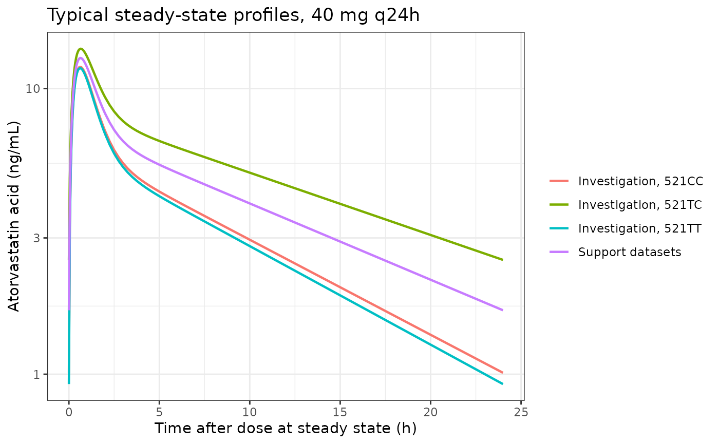
Closed-form check: AUC over the dosing interval
At steady state the AUC over one dosing interval equals F x Dose / CL (F is absorbed into the apparent CL/F). The typical CL/F values are 535, 535 x (1 - 0.402) = 319.9, 535 x (1 - 0.041) = 513.1 and 400 L/h. With dose in mg, CL in L/h and concentrations in ng/mL, AUC(0-24) = 1000 x Dose / CL.
typ_auc <- sim_typ |>
  dplyr::group_by(group) |>
  dplyr::summarise(
    cl = dplyr::first(cl),
    auc_trap = sum(diff(time) * (head(Cc, -1) + tail(Cc, -1)) / 2),
    .groups = "drop"
  ) |>
  dplyr::mutate(
    cl_expected = c(
      "Investigation, 521TT" = 535,
      "Investigation, 521TC" = 535 * (1 - 0.402),
      "Investigation, 521CC" = 535 * (1 - 0.041),
      "Support datasets" = 400
    )[group],
    auc_expected = 1000 * 40 / cl_expected,
    pct_diff = 100 * (auc_trap - auc_expected) / auc_expected
  )
typ_auc |>
  dplyr::rename(
    "Group" = group,
    "CL/F in model (L/h)" = cl,
    "CL/F from Table 3 (L/h)" = cl_expected,
    "AUC0-24 simulated (ng h/mL)" = auc_trap,
    "1000 x Dose / CL (ng h/mL)" = auc_expected,
    "% difference" = pct_diff
  ) |>
knitr::kable(digits = 2)| Group | CL/F in model (L/h) | AUC0-24 simulated (ng h/mL) | CL/F from Table 3 (L/h) | 1000 x Dose / CL (ng h/mL) | % difference |
|---|---|---|---|---|---|
| Investigation, 521CC | 513.07 | 77.96 | 513.06 | 77.96 | 0 |
| Investigation, 521TC | 319.93 | 125.03 | 319.93 | 125.03 | 0 |
| Investigation, 521TT | 535.00 | 74.77 | 535.00 | 74.77 | 0 |
| Support datasets | 400.00 | 100.00 | 400.00 | 100.00 | 0 |
Virtual cohort
A virtual investigation cohort
(STUDY_ATORVA_SUPPORT = 0) at the four most common
once-daily doses in Table 1 (10, 20, 40 and 80 mg), 200 patients per
dose. SLCO1B1 c.521T>C genotypes are assigned deterministically in
the proportions observed among the 65 genotyped patients (TT 44 : TC 16
: CC 5, Table 2). The model has no continuous covariates.
n_per_arm <- 200
doses <- c(10, 20, 40, 80)
geno <- c(
  rep("TT", round(n_per_arm * 44 / 65)),
  rep("TC", round(n_per_arm * 16 / 65))
)
geno <- c(geno, rep("CC", n_per_arm - length(geno)))

cohort <- tidyr::crossing(dose = doses, idx = seq_len(n_per_arm)) |>
  dplyr::mutate(
    id = dplyr::row_number(),
    genotype = geno[idx],
    STUDY_ATORVA_SUPPORT = 0,
    SNP_SLCO1B1_RS4149056_HET = as.integer(genotype == "TC"),
    SNP_SLCO1B1_RS4149056_HOM = as.integer(genotype == "CC"),
    treatment = paste(dose, "mg q24h")
  )
table(cohort$genotype, cohort$treatment)
#>
#>      10 mg q24h 20 mg q24h 40 mg q24h 80 mg q24h
#>   CC         16         16         16         16
#>   TC         49         49         49         49
#>   TT        135        135        135        135
obs_cohort <- sort(unique(c(
  0, 0.05, 0.1, 0.15, 0.2, 0.3, 0.4, 0.5, 0.6, 0.8, 1, 1.25, 1.5, 2, 2.5,
  3, 4, 5, 6, 8, 10, 12, 14, 16, 18, 20, 22, 24
)))
ev_list <- lapply(split(cohort, cohort$dose), function(d) {
  make_events(
    dplyr::select(
      d, id, STUDY_ATORVA_SUPPORT, SNP_SLCO1B1_RS4149056_HET,
      SNP_SLCO1B1_RS4149056_HOM
    ),
    dose = d$dose[1],
    obs_times = obs_cohort
  )
})
ev_cohort <- dplyr::bind_rows(ev_list) |>
  dplyr::arrange(id, time, dplyr::desc(evid))

rxode2::rxSetSeed(20220301)
sim <- rxode2::rxSolve(mod, ev_cohort, returnType = "data.frame", maxsteps = 1e6) |>
  dplyr::left_join(dplyr::select(cohort, id, dose, genotype, treatment), by = "id")
#> ℹ parameter labels from comments will be replaced by 'label()'
Concentration-time profiles at steady state
The paper’s pcVPC (Figure 3a; dose-stratified in Supplementary Figure
S1) plots sparse samples taken 2.2-40 h after the self-reported intake.
The figure below shows the simulated 5th, 50th and 95th percentiles of
the population prediction (Cc, no residual error) and of
the simulated observation (sim, with exponential residual
error) over one steady-state dosing interval.
vpc <- sim |>
  dplyr::group_by(treatment, time) |>
  dplyr::summarise(
    p05 = quantile(sim, 0.05), p50 = median(sim), p95 = quantile(sim, 0.95),
    c50 = median(Cc),
    .groups = "drop"
  ) |>
  dplyr::mutate(treatment = factor(treatment, levels = paste(doses, "mg q24h")))

ggplot(vpc, aes(time)) +
  geom_ribbon(aes(ymin = p05, ymax = p95), alpha = 0.25, fill = "steelblue") +
  geom_line(aes(y = p50), colour = "steelblue") +
  geom_line(aes(y = c50), colour = "black", linetype = "dashed") +
  facet_wrap(~treatment) +
  scale_y_log10() +
  labs(
    x = "Time after dose at steady state (h)",
    y = "Atorvastatin acid (ng/mL)",
    title = "Simulated steady-state percentiles (5th-95th band, median)",
    caption = "Compare with Figure 3a and Supplementary Figure S1 of Stillemans 2022."
  ) +
  theme_bw()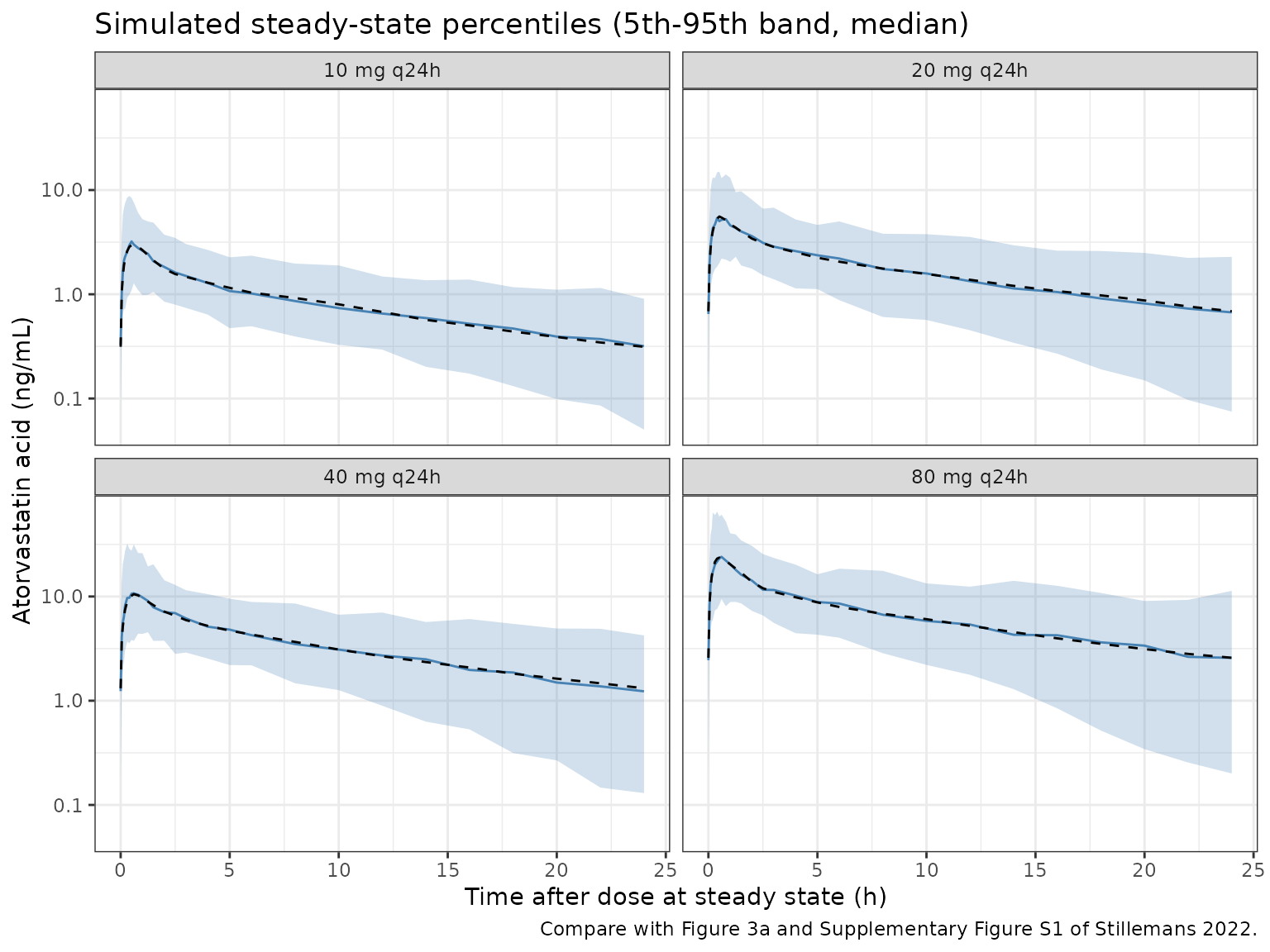
Individual CL/F by genotype
Figure 1c of the paper shows the individual (empirical Bayes) CL/F by SLCO1B1 c.521T>C genotype. The simulated CL/F distribution by genotype is shown for comparison; the paper’s EBEs are shrunk towards the typical value (shrinkage 44.3%), so the simulated spread is wider.
cl_ind <- sim |>
  dplyr::distinct(id, genotype, cl) |>
  dplyr::mutate(genotype = factor(genotype, levels = c("TT", "TC", "CC")))

ggplot(cl_ind, aes(genotype, cl)) +
  geom_boxplot() +
  geom_hline(yintercept = 414.67, linetype = "dotted") +
  labs(
    x = "SLCO1B1 c.521T>C genotype",
    y = "Individual CL/F (L/h)",
    caption = paste(
      "Dotted line: the paper's ROC-derived myalgia threshold, 414.67 L/h.",
      "Compare with Figure 1c."
    )
  ) +
  theme_bw()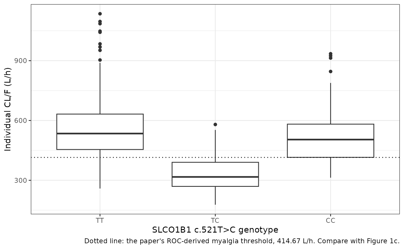
cl_ind |>
  dplyr::group_by(genotype) |>
  dplyr::summarise(
    n = dplyr::n(),
    median_cl = median(cl),
    pct_below_threshold = 100 * mean(cl < 414.67),
    .groups = "drop"
  ) |>
  dplyr::rename(
    "Genotype" = genotype,
    "N" = n,
    "Median CL/F (L/h)" = median_cl,
    "% with CL/F < 414.67 L/h" = pct_below_threshold
  ) |>
knitr::kable(digits = 1)| Genotype | N | Median CL/F (L/h) | % with CL/F < 414.67 L/h |
|---|---|---|---|
| TT | 540 | 534.5 | 15.7 |
| TC | 196 | 316.9 | 81.6 |
| CC | 64 | 504.3 | 25.0 |
# The median individual CL/F of each genotype stratum sits at its typical
# value (log-normal eta, median exp(0) = 1). Centre, not tails; the 15%
# bound leaves room for the sampling error of the 64-patient CC median
# (about 4%) while still catching the 40% TC effect being dropped.
cl_med <- cl_ind |>
  dplyr::group_by(genotype) |>
  dplyr::summarise(med = median(cl), .groups = "drop")
cl_typ <- c(TT = 535, TC = 535 * (1 - 0.402), CC = 535 * (1 - 0.041))
stopifnot(all(abs(cl_med$med / cl_typ[as.character(cl_med$genotype)] - 1) < 0.15))
NCA with PKNCA
The paper reports no NCA parameters (the investigation data are one sample per visit), so the NCA below characterises the simulated steady-state dosing interval and checks it against the closed-form identity AUC(0-24, ss) x CL/F = 1000 x Dose for each simulated patient, using that patient’s own CL/F.
conc_df <- sim |>
  dplyr::filter(!is.na(Cc)) |>
  dplyr::select(id, time, Cc, treatment)

dose_df <- cohort |>
  dplyr::transmute(id, time = 0, amt = dose, treatment)

conc_obj <- PKNCA::PKNCAconc(conc_df, Cc ~ time | treatment + id)
dose_obj <- PKNCA::PKNCAdose(dose_df, amt ~ time | treatment + id)
intervals <- data.frame(
  start = 0, end = 24,
  cmax = TRUE, tmax = TRUE, cmin = TRUE, auclast = TRUE, cav = TRUE
)
nca_res <- PKNCA::pk.nca(PKNCA::PKNCAdata(conc_obj, dose_obj, intervals = intervals))
nca_summary <- summary(nca_res)
knitr::kable(nca_summary)| start | end | treatment | N | auclast | cmax | cmin | tmax | cav |
|---|---|---|---|---|---|---|---|---|
| 0 | 24 | 10 mg q24h | 200 | 21.7 [31.4] | 3.20 [60.7] | 0.291 [107] | 0.600 [0.100, 1.50] | 0.904 [31.4] |
| 0 | 24 | 20 mg q24h | 200 | 42.2 [35.6] | 5.79 [56.2] | 0.537 [132] | 0.800 [0.100, 1.50] | 1.76 [35.6] |
| 0 | 24 | 40 mg q24h | 200 | 85.0 [34.0] | 11.4 [59.8] | 1.04 [168] | 0.800 [0.150, 1.50] | 3.54 [34.0] |
| 0 | 24 | 80 mg q24h | 200 | 168 [37.7] | 24.3 [53.9] | 2.05 [186] | 0.600 [0.100, 1.50] | 6.99 [37.7] |
auc_ind <- as.data.frame(nca_res) |>
  dplyr::filter(PPTESTCD == "auclast") |>
  dplyr::select(id, auclast = PPORRES) |>
  dplyr::left_join(dplyr::distinct(sim, id, cl, dose), by = "id") |>
  dplyr::mutate(
    expected = 1000 * dose / cl,
    pct_diff = 100 * (auclast - expected) / expected
  )

auc_ind |>
  dplyr::summarise(
    median_pct_diff = median(pct_diff),
    p90_abs_pct_diff = quantile(abs(pct_diff), 0.9)
  ) |>
knitr::kable(digits = 2)| median_pct_diff | p90_abs_pct_diff |
|---|---|
| 0.02 | 0.1 |
Assumptions and deviations
-
Omega and sigma scale. Table 3 labels the
variability rows “(SD)”, but the printed estimates are variances (see
“Omega and sigma scale” above); they are entered in
ini()as variances, and the residual SD is sqrt(0.085) = 0.2915. - CL/F variance of the investigation cohort. The Results text value 0.0677 is used; Table 3 prints the same quantity rounded to 0.068.
-
Residual error form. The paper states an
exponential residual error model, encoded as
lnorm(expSd)(additive on the log scale). -
Cohort split. The two CL/F typical values and
random effects are selected by
STUDY_ATORVA_SUPPORT. The support datasets had no genotype information (coded as missing), so the SLCO1B1 effect applies only whenSTUDY_ATORVA_SUPPORT = 0. For simulating the real-life ambulatory population the paper targets, setSTUDY_ATORVA_SUPPORT = 0. - SLCO1B1 521CC effect. The CC estimate (-0.041, RSE 469.7%) is the paper’s estimate and is kept as published even though the authors describe it as very imprecise and weaker than the heterozygous effect.
-
Screened covariates. OATP2B1-inhibitor
co-medication and sex entered the forward search but were removed at
backward elimination; the paper reports no final-model coefficient for
them. They are documented in
covariatesDataExcludedand are not part of the model. - Linear PK. The paper could not evaluate dose-linearity with the available data; the model is linear, as published.
- PK/PD relationships not packaged. The paper relates individual CL/F to creatine kinase (linear regression, slope -0.20 per L/h), myalgia (logistic regression, OR 0.68 per 50 L/h; ROC threshold 414.67 L/h) and the change in total and LDL cholesterol (correlations). Intercepts are not reported and the regressions are on post-hoc CL/F rather than on a simulated exposure, so they cannot be encoded as a simulatable PD model.
-
Virtual cohort. Genotype proportions come from the
65 genotyped investigation-cohort patients; doses are the four most
common regimens in Table 1. Steady state is reached with an
ss = 1dose record. - No published NCA. The paper reports no Cmax, AUC or half-life, so no side-by-side NCA comparison is possible; the NCA is checked against the closed-form dose/CL identity instead.