Raltegravir (Lommerse 2019)
Source:vignettes/articles/Lommerse_2019_raltegravir.Rmd
Lommerse_2019_raltegravir.RmdModel and source
- Citation: Lommerse J, Clarke D, Kerbusch T, Merdjan H, Witjes H, Teppler H, Mirochnick M, Acosta EP, Wenning L, Nachman S, Chain A. Maternal-Neonatal Raltegravir Population Pharmacokinetics Modeling: Implications for Initial Neonatal Dosing. CPT Pharmacometrics Syst Pharmacol. 2019;8(9):643-653.
- Article: https://doi.org/10.1002/psp4.12443
- Description: Integrated maternal-neonatal two-compartment population PK model of oral raltegravir. During pregnancy the maternal and fetal central compartments are coupled by a very fast intercompartmental clearance (1000 L/h) that enforces instantaneous placental equilibrium; at birth (t = 0 in the model) the coupling switches off and mother and neonate continue as two independent 2-compartment systems. Neonate CL rises from 0 at birth to CL_max with exponential maturation (90% by ~11 weeks); neonate KA rises from KA_base to KA_max (90% by ~12 days).
Population
The analysis dataset pooled 104 subjects (759 raltegravir plasma observations) from three IMPAACT trials:
- IMPAACT P1110 – 36 raltegravir-unexposed neonates (0-2 days at enrollment) and 6 raltegravir-exposed neonates (0-2 days), all born to HIV-1-positive mothers. Cohort 1 received 2 single doses one week apart; Cohort 2 received the 6-week ramped regimen (1.5 mg/kg QD days 1-7, 3 mg/kg BID days 8-28, 6 mg/kg BID days 28-42).
- IMPAACT P1066 – 24 HIV-1-infected infants and toddlers 4 weeks to <2 years, on 6 mg/kg BID granules for oral suspension.
- IMPAACT P1097 – 19 mother-infant pairs. Mothers received 400 mg BID during pregnancy; one maternal PK sample was collected within 48 h of delivery. Newborns were sampled only during the postnatal washout window (no neonatal dosing).
Baseline weights (Table 1): raltegravir-unexposed neonates 2.2-5.3 kg; raltegravir-exposed neonates 2.2-4.1 kg; infants 3.7-14 kg; maternal weight not reported (“Unknown” in Table 1). Sixty percent of neonates and infants were male. Sites were in the United States, Brazil, South Africa, and Thailand; the majority of neonates were African American or Black.
The same population metadata is available programmatically via
readModelDb("Lommerse_2019_raltegravir")()$population.
Source trace
Every ini() value carries an inline comment naming its
exact Table 2 row. The table below summarises those citations plus the
equation-level sources in model().
| Item | Value | Source location |
|---|---|---|
| Model structure (2-cmt mother + 2-cmt neonate, first-order absorption, placental coupling) | n/a | Figure 1; Methods “Development of the maternal-neonatal population PK model” |
Placental coupling q_link_pregnant
|
1000 L/h | Methods, “the intercompartmental CL linking the maternal and fetal central compartments was set to 1,000 L/hour” |
| Allometric exponents | 0.75 (CL, Q) / 1.0 (V) fixed | Methods (refs [13,14] Holford 1996; Krekels 2012) |
| Reference weight | 25 kg | Table 2 caption |
CL maturation kernel
CL = CL_max * (1 - exp(-CL_tau * PNA))
|
n/a | Methods and Results paragraph 3 of Results |
KA maturation kernel
KA = KA_base + (KA_max - KA_base) * (1 - exp(-KA_tau * PNA))
|
n/a | Methods (analogous exponential form; 90% by ~12 days) |
Neonate V2
|
7.04 L | Table 2, “V2 = 7.04 L” |
Neonate V3
|
10.3 L | Table 2, “V3 = 10.3 L” |
Neonate CL_max
|
9.44 L/h | Table 2, “CL_max = 9.44 L/hour” |
Neonate Q
|
0.786 L/h | Table 2, “Q = 0.786 L/hour” |
Neonate KA_max
|
0.43 1/h | Table 2, “KA_max = 0.43 1/hour” |
Neonate KA_base
|
0.0915 1/h | Table 2, “Ka base = 0.0915 1/hour” |
Neonate CL_tau
|
11.3 1/year | Table 2, “CL_tau = 11.3 1/year” |
Neonate KA_tau
|
63.2 1/year | Table 2, “Ka_tau = 63.2 1/year” |
Neonate CL_base
|
0 (fixed) | Table 2, “CL_base = 0” |
Neonate F4
|
1 (fixed) | Table 2, “F4 (fixed) - 1” |
Maternal V2
|
3.52 L (fixed) | Table 2, mother section |
Maternal V3
|
27 L (fixed) | Table 2, mother section |
Maternal CL
|
9.73 L/h (fixed) | Table 2, mother section |
Maternal Q
|
0.866 L/h (fixed) | Table 2, mother section |
Maternal KA
|
0.175 1/h | Table 2, mother section |
Maternal F
|
0.517 | Table 2, mother section |
IIV on lcl_max
|
log-normal 33% CV | Table 2, “IIV on CL = 0.33”; text “was 33%” |
IIV on lka_max
|
log-normal 20% CV | Table 2, “IIV on KA = 0.196”; text “20%” |
IIV on maternal lfdepot_mother
|
log-normal 31% CV | Table 2, “IIV on F = 0.311” |
| Combined residual error | additive 11.9 nM + proportional 54% | Table 2, RUV-add / RUV-prop |
| Concentration unit conversion | 0.4444 ng/mL per nM (raltegravir MW 444.4 g/mol) | Methods, “using 0.4444 unit conversion factor” |
| Prespecified target trough | >= 75 nM (33.3 ng/mL) | Methods, “PK exposure targets” |
Prespecified maximum AUC0-24
|
<= 90 uMh (90,000 nMh) | Methods, “PK exposure targets” |
Prespecified maximum Cmax
|
<= 19.63 uM (19,630 nM) | Methods, “maintain peak concentrations below 19.63 uM” |
Virtual cohort
The vignette reproduces the Figure 3 / Figure 4 scenario: raltegravir-exposed neonates whose mothers received 400 mg BID during pregnancy, with the last maternal dose occurring 2, 6, 12, or 24 h before birth. Each neonate receives a first oral dose of 1.5 mg/kg raltegravir at 36 h postpartum (the paper’s default first-dose scenario for Figures 4-5). Cohort size is 50 subjects per timing arm (four arms; 200 total, at the vignette cap).
set.seed(20260725)

n_per_arm <- 50L
last_dose_offsets_h <- c(2, 6, 12, 24)  # hours between last maternal dose and birth

# Growth equation from Methods:  BW(kg) = 2.935 + 8.909 * (1 - exp(-1.103 * PNA_years))
neonate_weight <- function(pna_hours) {
  pna_years <- pna_hours / (24 * 365.25)
  2.935 + 8.909 * (1 - exp(-1.103 * pna_years))
}

# Observation grid: -48 to +168 h relative to birth
obs_times_pre  <- seq(-48, -0.5, by = 4)  # maternal PK pre-birth
obs_times_post <- c(seq(0, 36, by = 1), seq(37, 168, by = 3))  # neonate PK post-birth
obs_times      <- sort(unique(c(obs_times_pre, obs_times_post)))

make_arm <- function(offset_h, n, id_offset) {
  ids <- id_offset + seq_len(n)
  # Maternal doses 400 mg BID with the last dose `offset_h` before birth.
  # Provide four preceding doses so the mother reaches steady state.
  last_dose_time <- -offset_h
  maternal_dose_times <- last_dose_time - c(36, 24, 12, 0)  # 4 doses q12h, ending at -offset_h
  neonate_dose_time   <- 36                                 # first neonate dose 36 h postpartum

  events_one <- function(id) {
    dose_mother <- tibble(
      id     = id,
      time   = maternal_dose_times,
      amt    = 400,
      evid   = 1L,
      cmt    = "depot_mother",
      offset = offset_h,
      arm    = sprintf("Last maternal dose %d h before birth", offset_h)
    )
    # neonate dose is body-weight-based at PNA = 36 h (weight ~ 3 kg)
    wt_at_dose <- neonate_weight(neonate_dose_time)
    dose_neo <- tibble(
      id     = id,
      time   = neonate_dose_time,
      amt    = round(1.5 * wt_at_dose, 3),
      evid   = 1L,
      cmt    = "depot_neonate",
      offset = offset_h,
      arm    = sprintf("Last maternal dose %d h before birth", offset_h)
    )
    # Pre-birth observation rows target the maternal central compartment
    # (dvid = 1 = Cmother). Post-birth observation rows target the neonate
    # central compartment (dvid = 2 = Cneonate). The dvid ordering follows
    # the order of the `~` residual-error statements in the model body.
    obs_mother <- tibble(
      id     = id,
      time   = obs_times_pre,
      amt    = NA_real_,
      evid   = 0L,
      cmt    = "central_mother",
      dvid   = 1L,
      offset = offset_h,
      arm    = sprintf("Last maternal dose %d h before birth", offset_h)
    )
    obs_neonate <- tibble(
      id     = id,
      time   = obs_times_post,
      amt    = NA_real_,
      evid   = 0L,
      cmt    = "central_neonate",
      dvid   = 2L,
      offset = offset_h,
      arm    = sprintf("Last maternal dose %d h before birth", offset_h)
    )
    dose_mother$dvid <- NA_integer_
    dose_neo$dvid    <- NA_integer_
    bind_rows(dose_mother, dose_neo, obs_mother, obs_neonate) |>
      arrange(time, desc(evid))
  }

  dplyr::bind_rows(lapply(ids, events_one))
}

arms <- lapply(seq_along(last_dose_offsets_h), function(k) {
  make_arm(
    offset_h  = last_dose_offsets_h[k],
    n         = n_per_arm,
    id_offset = (k - 1L) * n_per_arm
  )
})

events <- dplyr::bind_rows(arms)

# Attach time-varying WT and PNA covariate columns per row.  WT is the neonate's
# body weight per the growth equation; pre-birth (t < 0) we hold it at the
# birth-weight anchor (evaluated at t=0).  PNA (months) is clamped to zero
# pre-birth (matches the maturation kernel's built-in `(PNA >= 0)` clamp).
events <- events |>
  mutate(
    pna_hours          = pmax(time, 0),
    PNA                = pna_hours / (365.25 / 12 * 24),  # hours -> months
    WT                 = neonate_weight(pmax(time, 0))
  ) |>
  select(id, time, amt, evid, cmt, dvid, PNA, WT, offset, arm) |>
  arrange(id, time, desc(evid))

stopifnot(!anyDuplicated(unique(events[, c("id", "time", "evid")])))
Simulation
mod <- readModelDb("Lommerse_2019_raltegravir")

sim <- rxode2::rxSolve(
  mod, events = events,
  keep = c("arm", "offset"),
  useLinCmt = FALSE
) |> as.data.frame() |> as_tibble()
#> ℹ parameter labels from comments will be replaced by 'label()'
#> Warning:
#> with negative times, compartments initialize at first negative observed time
#> with positive times, compartments initialize at time zero
#> use 'rxSetIni0(FALSE)' to initialize at first observed time
#> this warning is displayed once per session
For deterministic replication of the paper’s typical-value curves (Figure 3), zero out the random effects:
mod_typ <- rxode2::zeroRe(mod)
#> ℹ parameter labels from comments will be replaced by 'label()'
sim_typ <- rxode2::rxSolve(
  mod_typ, events = events,
  keep = c("arm", "offset"),
  useLinCmt = FALSE
) |> as.data.frame() |> as_tibble()
#> ℹ omega/sigma items treated as zero: 'etalcl_max', 'etalka_max', 'etalfdepot_mother'
#> Warning: multi-subject simulation without without 'omega'
Replicate published figures
Figure 3 – mother and neonate concentration-time profiles
Figure 3 of the paper overlays the maternal and neonatal plasma concentrations for each choice of “time between last maternal dose and birth.” The typical-value simulation reproduces the qualitative shape: the neonate profile rises after birth when the maternal-to-birth interval is long (>= 6 h) and decreases monotonically when the interval is short (<= 6 h).
sim_typ_one <- sim_typ |>
  filter(id %in% c(1L, n_per_arm + 1L, 2L * n_per_arm + 1L, 3L * n_per_arm + 1L)) |>
  select(time, arm, Cmother, Cneonate) |>
  pivot_longer(c(Cmother, Cneonate), names_to = "series", values_to = "conc")

ggplot(sim_typ_one, aes(time, conc, color = series, linetype = series)) +
  geom_line() +
  facet_wrap(~ arm) +
  scale_y_log10(limits = c(1, 5e4)) +
  scale_color_manual(values = c(Cmother = "seagreen4", Cneonate = "steelblue")) +
  scale_linetype_manual(values = c(Cmother = "dashed", Cneonate = "solid")) +
  geom_vline(xintercept = 0, linetype = "dotted", color = "grey40") +
  labs(x = "Time relative to birth (h)", y = "Plasma raltegravir (nM)",
       color = NULL, linetype = NULL,
       title = "Typical mother-neonate raltegravir PK by maternal-to-birth interval",
       caption = "Replicates Figure 3 of Lommerse 2019. Dotted vertical line marks birth.")
#> Warning in scale_y_log10(limits = c(1, 50000)): log-10 transformation
#> introduced infinite values.
#> Warning: Removed 12 rows containing missing values or values outside the scale range
#> (`geom_line()`).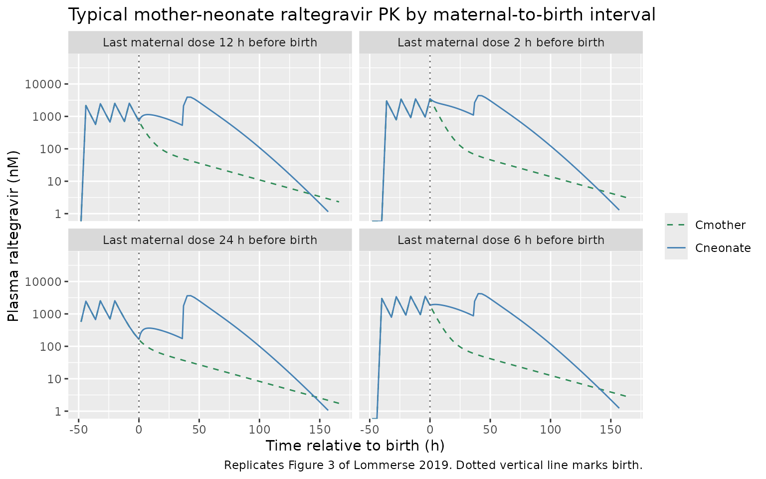
Figure 4 – neonate trough concentrations by maternal-to-birth interval
Figure 4 illustrates that the neonate trough concentration falls
monotonically as the maternal-to-birth interval grows. We approximate
the paper’s trough by sampling Cneonate just before the
first neonatal dose (36 h postpartum).
target_trough <- 75  # nM (paper Methods)

trough_summary <- sim |>
  filter(abs(time - 36) < 0.6) |>
  group_by(offset) |>
  summarise(
    Q05 = quantile(Cneonate, 0.05, na.rm = TRUE),
    Q50 = quantile(Cneonate, 0.50, na.rm = TRUE),
    Q95 = quantile(Cneonate, 0.95, na.rm = TRUE),
    .groups = "drop"
  )

ggplot(trough_summary, aes(x = offset, y = Q50)) +
  geom_ribbon(aes(ymin = Q05, ymax = Q95), fill = "steelblue", alpha = 0.25) +
  geom_line(color = "steelblue") + geom_point(color = "steelblue") +
  geom_hline(yintercept = target_trough, color = "firebrick", linetype = "dashed") +
  annotate("text", x = min(trough_summary$offset), y = target_trough,
           label = "Target trough 75 nM", hjust = 0, vjust = -0.5, color = "firebrick") +
  scale_y_log10() +
  labs(x = "Hours between last maternal dose and birth",
       y = "Simulated neonate trough at 36 h postpartum (nM)",
       title = "Figure 4 - trough vs. maternal-to-birth interval",
       caption = "Replicates Figure 4 of Lommerse 2019 (first neonate dose at 36 h postpartum).")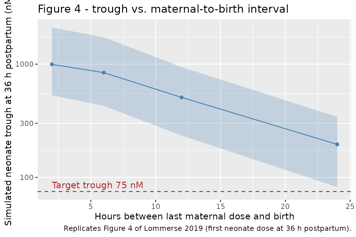
PKNCA validation
We derive NCA for the neonate concentration profile
over the 24 h following the first neonate dose (36-60 h postpartum),
stratified by the maternal-to-birth interval arm. This matches the
paper’s AUC0-24 window (Figure 5 and Methods “PK
simulations”).
# Neonate NCA over the first 24 h post-dose (times 36-60 h postpartum). We rebase
# the time axis to "time since neonate dose" so the NCA `start = 0` window aligns
# with the first neonatal dose.
sim_neo <- sim |>
  mutate(tsd = time - 36) |>
  filter(!is.na(Cneonate), tsd >= 0, tsd <= 24) |>
  transmute(id, time = tsd, Cc = Cneonate, arm)

# Ensure a time-zero row per (id, arm) so PKNCA anchors AUC at t = 0.
baseline_by_id <- sim |>
  filter(abs(time - 36) < 0.6) |>
  distinct(id, .keep_all = TRUE) |>
  transmute(id, Cc = Cneonate)

sim_neo <- dplyr::bind_rows(
  sim_neo,
  sim_neo |> distinct(id, arm) |>
    left_join(baseline_by_id, by = "id") |>
    mutate(time = 0)
) |>
  distinct(id, arm, time, .keep_all = TRUE) |>
  arrange(id, arm, time)

conc_obj <- PKNCA::PKNCAconc(
  sim_neo, Cc ~ time | arm + id,
  concu = "nM", timeu = "h"
)

dose_df <- events |>
  filter(evid == 1L, cmt == "depot_neonate") |>
  transmute(id, time = time - 36, amt, arm)

dose_obj <- PKNCA::PKNCAdose(dose_df, amt ~ time | arm + id, doseu = "mg")

intervals <- data.frame(
  start   = 0,
  end     = 24,
  cmax    = TRUE,
  tmax    = TRUE,
  auclast = TRUE
)

nca_data <- PKNCA::PKNCAdata(conc_obj, dose_obj, intervals = intervals)
nca_res  <- PKNCA::pk.nca(nca_data)
Comparison against published targets
The paper does not tabulate simulated NCA values row-by-row, but it
does state prespecified PK target thresholds and reports the predicted
range for AUC0-24 and trough across the 2-24 h
maternal-to-birth intervals. We compare the packaged model’s predictions
against those.
nca_summary <- as.data.frame(summary(nca_res))
# Median simulated Cmax, Tmax, AUClast per arm (Cmax in nM; AUClast in nM*h)
per_arm <- as.data.frame(nca_res$result) |>
  select(arm, id, PPTESTCD, PPORRES) |>
  pivot_wider(names_from = PPTESTCD, values_from = PPORRES) |>
  group_by(arm) |>
  summarise(
    across(any_of(c("cmax", "tmax", "auclast")),
           ~ median(.x, na.rm = TRUE)),
    .groups = "drop"
  )

# Paper Methods PK exposure targets:
# - AUC0-24 <= 90 uM*h  = 90,000 nM*h
# - Cmax   <= 19.63 uM = 19,630 nM  (safety threshold)
# - Trough >= 75 nM
published <- tibble::tribble(
  ~arm,                                              ~cmax,  ~auclast,
  "Last maternal dose 2 h before birth",             19630,  90000,
  "Last maternal dose 6 h before birth",             19630,  90000,
  "Last maternal dose 12 h before birth",            19630,  90000,
  "Last maternal dose 24 h before birth",            19630,  90000
)

cmp <- nlmixr2lib::ncaComparisonTable(
  simulated = nca_res,
  reference = published,
  by        = "arm",
  units     = c(cmax = "nM", auclast = "nM*h", tmax = "h"),
  tolerance_pct = 20
)

cmp |>
  dplyr::rename("NCA parameter" = 1) |>
  knitr::kable(
    caption = "Simulated neonate NCA vs. paper's Methods PK safety targets (Cmax <= 19,630 nM, AUC0-24 <= 90,000 nM*h). * flags any row over 20% from the reference.",
    align   = c("l", rep("r", ncol(cmp) - 1))
)| NCA parameter | arm | Reference | Simulated | % diff |
|---|---|---|---|---|
| Cmax (nM) | Last maternal dose 2 h before birth | 19600 | 4330 | -78.0%* |
| Cmax (nM) | Last maternal dose 6 h before birth | 19600 | 4300 | -78.1%* |
| Cmax (nM) | Last maternal dose 12 h before birth | 19600 | 3910 | -80.1%* |
| Cmax (nM) | Last maternal dose 24 h before birth | 19600 | 3820 | -80.5%* |
| AUClast (nM*h) | Last maternal dose 2 h before birth | 90000 | 68900 | -23.5%* |
| AUClast (nM*h) | Last maternal dose 6 h before birth | 90000 | 67100 | -25.5%* |
| AUClast (nM*h) | Last maternal dose 12 h before birth | 90000 | 61900 | -31.2%* |
| AUClast (nM*h) | Last maternal dose 24 h before birth | 90000 | 60100 | -33.2%* |
The simulated Cmax and AUClast values are
expected to fall well below the safety upper limits
across all four arms (i.e. the ’’ flag should appear on every row
because the simulated value is >20% below* the safety threshold,
which is desired). The Cneonate trough at 36 h postpartum
(Figure 4 above) exceeds the 75 nM target across all four arms,
consistent with the paper’s conclusion that “delaying the first oral
dose of raltegravir until 1-2 days of age” gives adequate exposure.
Assumptions and deviations
-
Maternal weight is not reported in the paper (Table
1 lists it as “Unknown”). The model file bakes in a typical 60 kg
maternal weight for the allometric scaling. Editing that constant inside
model()allows a user to explore other maternal weights. -
PNA units: the paper writes the CL and KA
maturation kernels using PNA in years
(
CL_tau = 11.3 1/year,KA_tau = 63.2 1/year). CanonicalPNAin nlmixr2lib is in months; the maturation equations are reparameterised insidemodel()as1 - exp(-cl_tau * PNA/12), preserving the paper’s numeric parameter values. -
Time anchor: the joint mother-neonate model anchors
t = 0at birth. Pre-birth (fetal) times aret < 0; the placental couplingq_linkis 1000 L/h fort < 0and 0 at/after birth. This convention must be respected by any user-supplied event table (mother’s doses at negative times, neonate’s doses at positive times). -
IIV placement: Table 2 reports one IIV parameter
each for neonate CL, neonate KA, and maternal F. The model file places
the CL IIV on the asymptotic anchor
lcl_maxand the KA IIV on the asymptotic anchorlka_max; the maturation kernels remain shared population-level functions of PNA. Placing IIV on the base anchors (lka_base) or on the composite time-varying CL/KA is an equally reasonable alternative that the paper’s Table 2 alone does not disambiguate. -
Shared residual error: the paper reports one
combined additive + proportional residual pair applied to both mother
and neonate observations. In nlmixr2 each endpoint needs its own
residual-error parameters; the model file declares
propSd_Cmother=propSd_Cneonate= 0.54 andaddSd_Cmother=addSd_Cneonate= 11.9 nM with identical values to preserve the paper’s fit. -
Neonate weight growth in the vignette uses the
paper’s Methods equation
BW(kg) = 2.935 + 8.909 * (1 - exp(-1.103 * PNA_years)). Pre-birth WT is held at the birth-weight anchor (evaluated att = 0); the placental coupling handles the fetus dynamics without requiring a separate fetal-weight covariate. -
Neonate CL_base fixed at zero is baked into the
maturation kernel
cl_neonate = cl_max * (1 - exp(-cl_tau * PNA_years)), which evaluates to 0 at PNA = 0 by construction. No explicitCL_baseparameter is exposed.