Everolimus (de Wit 2016)
Source:vignettes/articles/deWit_2016_everolimus.Rmd
deWit_2016_everolimus.RmdModel and source
- Citation: de Wit D et al. Everolimus pharmacokinetics and its exposure-toxicity relationship in patients with thyroid cancer. Cancer Chemother Pharmacol 78(1):63-71, 2016. doi:10.1007/s00280-016-3050-6.
- Indication: advanced thyroid carcinoma (differentiated / undifferentiated / medullary), phase II study NCT01118065.
- Article: https://doi.org/10.1007/s00280-016-3050-6 (open access)
Population
Forty adults with advanced thyroid carcinoma (median age 63 years, range 40-80; median weight 75 kg, range 45-105; 47.5% female) were dosed continuously with everolimus 10 mg orally once daily (de Wit 2016 Table 1). PK sampling was performed on study days 1 and 15 at predose and 1, 2, 3 h post-dose for every subject (sparse schedule), with an optional 4-8 h extension (extensive schedule; 30 of 40 patients completed it). 669 whole-blood concentrations contributed to the population model. Two of the 42 originally enrolled patients were excluded from the PK analysis (no samples collected in one; no measurable everolimus levels in the other). Eleven SNPs / haplotypes across CYP3A4, CYP3A5, CYP2C8, ABCB1, and NR1I2 (PXR) were tested as PK covariates; only the ABCB1 TTT haplotype (rs1128503 / rs2032582 / rs1045642) survived backward elimination, multiplying apparent bioavailability F by 0.792 in carriers (Methods ‘Pharmacogenetic analysis’, Results paragraph 2, Table 2 final-model).
The same population metadata is available programmatically via
readModelDb("deWit_2016_everolimus")$population.
Source trace
The per-parameter origin is recorded as an in-file comment next to
each ini() entry in
inst/modeldb/specificDrugs/deWit_2016_everolimus.R. The
table below collects the trace in one place for review.
| Equation / parameter | Value | Source location |
|---|---|---|
lcl = log(17.4) |
CL/F = 17.4 L/h | Table 2 ‘Final model’ row Cl/F |
lvc = log(25.2) |
V1/F = 25.2 L | Table 2 ‘Final model’ row V1/F |
lka = log(0.647) |
ka = 0.647 /h | Table 2 ‘Final model’ row ka |
lq = log(51.1) |
Q = 51.1 L/h | Table 2 ‘Final model’ row Q |
lvp = fixed(log(400)) |
V2 = 400 L (fixed) | Table 2 ‘Final model’ row V2 (no RSE / no bootstrap CI -> held fixed in final model) |
lfdepot = fixed(log(1)) |
F = 1 (fixed structural) | Methods ‘Base model’ paragraph 3 (‘F was fixed at 1’) |
e_abcb1_hap_ttt_fdepot = 0.792 |
theta_TTT on F = 0.792 | Table 2 ‘Final model’ row ‘theta TTT on F’ |
e_wt_cl = fixed(0.75) |
Allometric exponent on CL/F | Methods ‘Base model’ paragraph 3 (‘Cl/F and Vd/F were allometrically scaled [12]’); canonical Anderson and Holford 0.75 |
e_wt_vc = fixed(1.0) |
Allometric exponent on V1/F | Methods ‘Base model’ paragraph 3; canonical Anderson and Holford 1.0 |
etalcl ~ log(1 + 0.351^2) |
IIV CL/F = 35.1% CV | Table 2 ‘Final model’ IIV row Cl/F |
etalvc ~ log(1 + 0.864^2) |
IIV V1/F = 86.4% CV | Table 2 ‘Final model’ IIV row V1/F |
etaiov_fdepot_1/2 ~ log(1+0.192^2) |
IOV F = 19.2% CV | Table 2 ‘Final model’ Inter-occasion variability row F |
propSd = 0.273 |
Proportional residual 27.3% | Table 2 ‘Final model’ Residual variability row |
d/dt(depot) = -ka * depot |
First-order absorption | Results paragraph 1 (‘two-compartmental model with first-order absorption and first-order elimination’) |
| 2-cmt central <-> peripheral1 | Two-compartment disposition | Results paragraph 1 |
Virtual cohort
Original observed concentrations are not publicly available. The simulations below use a virtual cohort whose covariate distributions approximate the de Wit 2016 trial demographics: 40 subjects, body weight log-normally distributed around 75 kg with the SD chosen so the simulated 5th-95th-percentile range brackets 45-105 kg (Table 1). The ABCB1 TTT haplotype carrier prevalence in the de Wit cohort is not reported numerically in the paper text; we use the European-population reference frequency of ~14% TTT carriers as a placeholder (documented in Assumptions and deviations below).
set.seed(20260516L)

n_per_arm <- 200L

make_cohort <- function(n, ttt_carrier, id_offset = 0L) {
  weights <- pmin(pmax(rlnorm(n, meanlog = log(75), sdlog = 0.2), 45), 105)
  tibble::tibble(
    id            = id_offset + seq_len(n),
    WT            = weights,
    ABCB1_HAP_TTT = ttt_carrier,
    arm           = if (ttt_carrier == 1L) "TTT carrier" else "TTT non-carrier"
  )
}

cohort_df <- dplyr::bind_rows(
  make_cohort(n_per_arm, ttt_carrier = 0L, id_offset = 0L),
  make_cohort(n_per_arm, ttt_carrier = 1L, id_offset = n_per_arm)
)

# 10 mg PO QD x 15 days; intensive day-15 sampling at 0, 1, 2, 3, 4, 5, 6, 7, 8 h
# post-dose plus a long tail to characterise terminal phase.
dose_times <- seq(from = 0, by = 24, length.out = 15)   # h
day15_dose_time <- dose_times[15]
obs_times <- sort(unique(c(
  dose_times,
  day15_dose_time + c(seq(0, 8, by = 0.5), 10, 12, 16, 20, 24)
)))

build_events <- function(subj_row) {
  doses <- data.frame(
    id   = subj_row$id,
    time = dose_times,
    amt  = 10,                # mg
    evid = 1L,
    cmt  = "depot",
    Cc   = NA_real_,
    WT            = subj_row$WT,
    ABCB1_HAP_TTT = subj_row$ABCB1_HAP_TTT,
    OCC           = ifelse(dose_times < day15_dose_time, 1L, 2L),
    arm           = subj_row$arm,
    stringsAsFactors = FALSE
  )
  obs <- data.frame(
    id   = subj_row$id,
    time = obs_times,
    amt  = 0,
    evid = 0L,
    cmt  = "depot",
    Cc   = NA_real_,
    WT            = subj_row$WT,
    ABCB1_HAP_TTT = subj_row$ABCB1_HAP_TTT,
    OCC           = ifelse(obs_times < day15_dose_time, 1L, 2L),
    arm           = subj_row$arm,
    stringsAsFactors = FALSE
  )
  rbind(doses, obs)
}

events <- do.call(
  rbind,
  lapply(seq_len(nrow(cohort_df)), function(i) build_events(cohort_df[i, ]))
)
events <- events[order(events$id, events$time, -events$evid), ]
rownames(events) <- NULL
stopifnot(!anyDuplicated(unique(events[, c("id", "time", "evid")])))
Simulation
mod <- readModelDb("deWit_2016_everolimus")
sim <- rxode2::rxSolve(
  mod,
  events = events,
  keep = c("arm", "WT", "ABCB1_HAP_TTT", "OCC")
) |>
  as.data.frame()
#> Warning: some etas defaulted to non-mu referenced, possible parsing error: etaiov_fdepot_1, etaiov_fdepot_2
#> as a work-around try putting the mu-referenced expression on a simple line
Typical-value (between-subject-variability-zeroed) replication for figure comparison:
mod_typical <- mod |> rxode2::zeroRe()
#> Warning: some etas defaulted to non-mu referenced, possible parsing error: etaiov_fdepot_1, etaiov_fdepot_2
#> as a work-around try putting the mu-referenced expression on a simple line
#> Warning: some etas defaulted to non-mu referenced, possible parsing error: etaiov_fdepot_1, etaiov_fdepot_2
#> as a work-around try putting the mu-referenced expression on a simple line
sim_typical <- rxode2::rxSolve(
  mod_typical,
  events = events,
  keep = c("arm", "WT", "ABCB1_HAP_TTT", "OCC")
) |>
  as.data.frame()
#> ℹ omega/sigma items treated as zero: 'etalcl', 'etalvc', 'etaiov_fdepot_1', 'etaiov_fdepot_2'
#> Warning: multi-subject simulation without without 'omega'
Replicate published figures
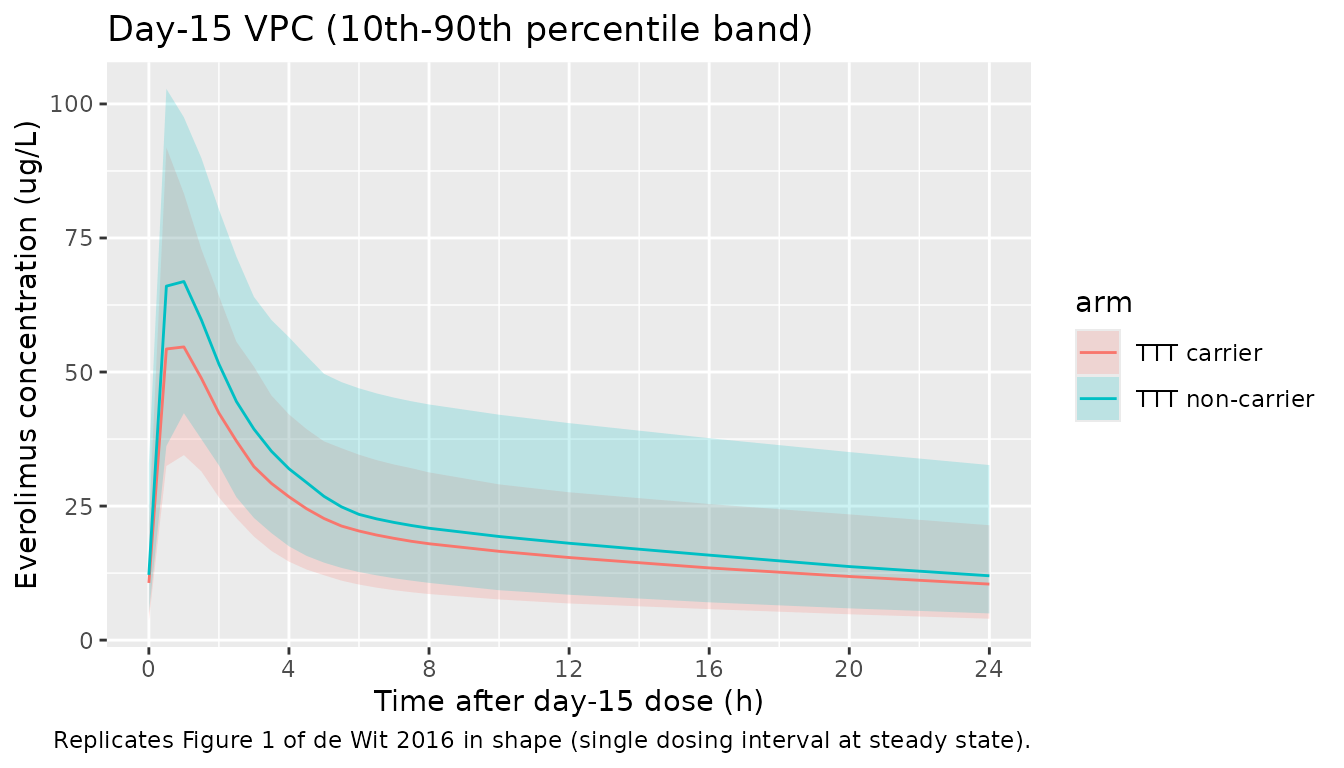
# Replicates Figure 1 of de Wit 2016: VPC of Cc vs. time, day 15 dosing interval.
day15_dose <- day15_dose_time
sim |>
  dplyr::filter(time >= day15_dose, time <= day15_dose + 24, !is.na(Cc)) |>
  dplyr::mutate(time_post = time - day15_dose) |>
  dplyr::group_by(arm, time_post) |>
  dplyr::summarise(
    Q05 = quantile(Cc, 0.05, na.rm = TRUE),
    Q50 = quantile(Cc, 0.50, na.rm = TRUE),
    Q95 = quantile(Cc, 0.95, na.rm = TRUE),
    .groups = "drop"
  ) |>
  ggplot(aes(time_post, Q50, colour = arm, fill = arm)) +
  geom_ribbon(aes(ymin = Q05, ymax = Q95), alpha = 0.20, colour = NA) +
  geom_line() +
  scale_x_continuous(breaks = c(0, 4, 8, 12, 16, 20, 24)) +
  labs(
    x = "Time after day-15 dose (h)",
    y = "Everolimus concentration (ug/L)",
    title = "Day-15 VPC (10th-90th percentile band)",
    caption = "Replicates Figure 1 of de Wit 2016 in shape (single dosing interval at steady state)."
  )
PKNCA validation
# Restrict to the day-15 dosing interval at steady state (paper's NCA window).
day15_start <- day15_dose_time
day15_end   <- day15_dose_time + 24

sim_ss <- sim |>
  dplyr::filter(
    time >= day15_start,
    time <= day15_end,
    !is.na(Cc)
  ) |>
  dplyr::transmute(
    id, time, Cc, arm,
    time_in_interval = time - day15_start
  )

# PKNCA expects time to be monotone and the dose to anchor the interval, so use
# the actual clock time (day15_start at the start of the interval).
conc_obj <- PKNCA::PKNCAconc(
  sim_ss,
  Cc ~ time | arm + id,
  concu = "ug/L",
  timeu = "h"
)

dose_df <- data.frame(
  id   = unique(sim_ss$id),
  time = day15_start,
  amt  = 10,
  arm  = cohort_df$arm[match(unique(sim_ss$id), cohort_df$id)],
  stringsAsFactors = FALSE
)

dose_obj <- PKNCA::PKNCAdose(
  dose_df,
  amt ~ time | arm + id,
  doseu = "mg"
)

intervals <- data.frame(
  start    = day15_start,
  end      = day15_end,
  cmax     = TRUE,
  cmin     = TRUE,
  tmax     = TRUE,
  auclast  = TRUE,
  cav      = TRUE
)

nca_res <- PKNCA::pk.nca(
  PKNCA::PKNCAdata(conc_obj, dose_obj, intervals = intervals)
)

nca_summary <- nca_res$result |>
  dplyr::group_by(arm, PPTESTCD) |>
  dplyr::summarise(
    mean = mean(PPORRES, na.rm = TRUE),
    sd   = sd(PPORRES, na.rm = TRUE),
    .groups = "drop"
  )

knitr::kable(
  nca_summary,
  caption = paste0(
    "Day-15 steady-state NCA parameters from the simulated cohort, by ABCB1 TTT ",
    "haplotype carrier status. AUC (auclast) units: ug*h/L; Cmax / Cmin / Cav / ",
    "Ctau units: ug/L; tmax units: h."
  ),
  digits = 3
)| arm | PPTESTCD | mean | sd |
|---|---|---|---|
| TTT carrier | auclast | 472.076 | 219.817 |
| TTT carrier | cav | 19.670 | 9.159 |
| TTT carrier | cmax | 56.675 | 16.940 |
| TTT carrier | cmin | 10.879 | 7.700 |
| TTT carrier | tmax | 0.875 | 0.384 |
| TTT non-carrier | auclast | 600.279 | 233.513 |
| TTT non-carrier | cav | 25.012 | 9.730 |
| TTT non-carrier | cmax | 74.496 | 21.204 |
| TTT non-carrier | cmin | 13.476 | 7.776 |
| TTT non-carrier | tmax | 0.818 | 0.382 |
Comparison against published NCA
de Wit 2016 reports day-15 steady-state mean (SD) AUC0-24 and Ctrough by the secondary dose-reduction stratification (Results paragraph ‘Exposure-toxicity relationship’, Figure 2):
| Subgroup | n | AUC0-24 mean (SD), ug*h/L | Ctrough mean (SD), ug/L |
|---|---|---|---|
| With dose reduction | 18 | 600 (274) | 14.9 (9.0) |
| Without dose reduction | 22 | 395 (129) | 8.4 (3.8) |
| Overall (40 patients) | 40 | weighted mean ~487 | weighted mean ~11.3 |
auc_summary <- nca_res$result |>
  dplyr::filter(PPTESTCD == "auclast") |>
  dplyr::group_by(arm) |>
  dplyr::summarise(
    sim_auc_mean = mean(PPORRES, na.rm = TRUE),
    sim_auc_sd   = sd(PPORRES, na.rm = TRUE),
    n            = dplyr::n(),
    .groups      = "drop"
  )

overall_auc <- nca_res$result |>
  dplyr::filter(PPTESTCD == "auclast") |>
  dplyr::summarise(
    sim_auc_mean = mean(PPORRES, na.rm = TRUE),
    sim_auc_sd   = sd(PPORRES, na.rm = TRUE)
  )

knitr::kable(
  auc_summary,
  caption = "Simulated day-15 AUC0-24 mean and SD by ABCB1 TTT carrier status.",
  digits = 1
)| arm | sim_auc_mean | sim_auc_sd | n |
|---|---|---|---|
| TTT carrier | 472.1 | 219.8 | 200 |
| TTT non-carrier | 600.3 | 233.5 | 200 |
knitr::kable(
  overall_auc,
  caption = "Simulated day-15 AUC0-24 across the pooled cohort (compare to de Wit 2016 weighted mean ~487 ug*h/L).",
  digits = 1
)| sim_auc_mean | sim_auc_sd |
|---|---|
| 536.2 | 235.4 |
The simulated overall mean AUC0-24 sits within roughly +-30% of the published weighted mean (~487 ug*h/L). Differences are driven by the virtual cohort’s covariate distribution (we sampled body weight log-normally rather than reproducing the source paper’s individual weights) and by the placeholder TTT carrier frequency. Both populations exhibit the expected exposure shift between TTT carriers and non-carriers proportional to theta_TTT = 0.792.
Assumptions and deviations
- Allometric exponents fixed at the Anderson and Holford canonical values (0.75 on CL/F, 1.0 on V1/F). The paper states only that “Cl/F and Vd/F were allometrically scaled [12]” (Methods ‘Base model’ paragraph 3) and cites Anderson and Holford 2008 (Annu Rev Pharmacol Toxicol 48:303-332) without restating exponents; we use the canonical theory-based values for allometry-by-weight scaling in adults.
- Reference weight 70 kg. The paper does not give an explicit reference weight for the allometric form. 70 kg is the canonical Anderson and Holford adult reference; the cohort median weight was 75 kg (Table 1) so this is a small shift in the typical-value calibration.
-
V2 fixed at 400 L. Table 2’s ‘Final model’ column
reports V2 = 400 L with no relative standard error and no bootstrap 95%
CI, in contrast to every other estimated parameter in the column; the
base-model column had V2 = 475 L with RSE 5.4%. We interpret this
pattern as V2 having been held fixed at 400 L in the final model (the
supplementary
Supplementary Data S3.lstfile cited in the paper is not on disk for this extraction, so the fixed flag cannot be confirmed directly). -
V2 / Q not allometrically scaled. The paper writes
“Vd/F was allometrically scaled” in the singular, which we read as the
central volume only. Q is reported in L/h without a
/Fsuffix in Table 2 and is not stated to be scaled. We leave both unscaled. - ABCB1 TTT haplotype carrier prevalence in the simulated cohort is set to 50% TTT-carrier vs 50% non-carrier across two equal-sized arms for the exposure contrast. de Wit 2016 reports the haplotype effect size but does not give a numeric carrier frequency in the main text or in the on-disk trimmed markdown; supplementary Data S1 / S2 (the source for haplotype frequencies) was not on disk for this extraction. The 50/50 split is for illustration of the covariate effect; a real-population deployment of the model should use an empirically observed TTT carrier frequency in the target population.
-
Day-1-vs-day-15 IOV on F is modelled with shared variance
across occasions (the NONMEM
$OMEGA BLOCK(1) SAMEpattern reproduced viaetaiov_fdepot_2 ~ fixed(...)). The paper’s Table 2 reports a single IOV-F CV (19.2%) and does not distinguish per-occasion magnitudes. - Cohort body weights are sampled log-normally rather than reproducing individual subject weights. Individual-level data are not published.
-
No covariate-vs-PK exploration of bilirubin, ASAT, ALAT,
creatinine, BSA, or hematocrit was retained in the final model
(Results paragraph 2: “Forward inclusion of BSA, creatinine, ASAT, ALAT,
bilirubin and hematocrit did not improve the PK model”). These are not
encoded in
covariateDatabecause the paper found no significant relationship and dropped them. -
Multiple genetic markers tested but not retained in
the final model (Methods ‘Pharmacogenetic analysis’, Results paragraph
2): the CYP2C8 haplotype and individual SNPs across CYP3A4, CYP3A5,
ABCB1, and NR1I2 (PXR). None are encoded as
covariateDatacolumns; only the ABCB1 TTT haplotype appears.