Emodepside (Assmus 2022) • nlmixr2lib

Model and source

Citation: Assmus F, Hoglund RM, Monnot F, Specht S, Scandale I, Tarning J. Drug development for the treatment of onchocerciasis: Population pharmacokinetic and adverse events modeling of emodepside. PLoS Negl Trop Dis. 2022;16(3):e0010219. doi:10.1371/journal.pntd.0010219. PMCID: PMC8912909. Parameter values from Table 3 and the S1 Code NONMEM control stream (supporting information).
Description: Three-compartment population PK model with a four-transit-compartment absorption chain (ka = ktr = 5/MTT) and linear elimination for oral emodepside in healthy male volunteers pooled from three phase I studies (single ascending dose, multiple ascending dose and relative bioavailability; Assmus 2022). CL/F, Q/F and Q2/F scale allometrically with body weight (exponent 0.75, reference 75 kg) and every volume linearly. Formulation (ASD-tablet A or B versus the oral liquid service formulation solution) and food act on both the mean transit time and the relative bioavailability, and the daily dose per kg body weight lengthens the mean transit time linearly. Inter-occasion variability on the mean transit time applies only to the two occasions of the multiple ascending dose study. Venous plasma (Cc) and dried-blood-spot (Cb) concentrations are linked by an estimated scaling factor of 0.618 and carry separate log-scale residual errors.
Article: https://doi.org/10.1371/journal.pntd.0010219 (open access, PLoS Neglected Tropical Diseases 16(3):e0010219)

Assmus 2022 developed the first population PK model of emodepside, an anthelmintic in development as a macrofilaricide for onchocerciasis (river blindness), and linked the model-predicted peak concentration to drug-related treatment-emergent adverse events (TEAEs) by binary logistic regression. The paper contributes five models to nlmixr2lib:

Model	What it predicts	Source
`Assmus_2022_emodepside`	Venous plasma (`Cc`) and dried-blood-spot (`Cb`) emodepside concentrations	Table 3; S1 Code
`Assmus_2022_emodepside_teae_interest`	Probability of a drug-related eye or nervous system disorder TEAE (the “TEAE of interest”)	S6 Table
`Assmus_2022_emodepside_eye_disorder`	Probability of a drug-related eye disorder TEAE	S6 Table
`Assmus_2022_emodepside_nervous_system_disorder`	Probability of a drug-related nervous system disorder TEAE	S6 Table
`Assmus_2022_emodepside_teae_drug_related`	Probability of any drug-related TEAE	S7 Table

The four logistic models take the individual maximum plasma concentration as a data column (CMAX, ng/mL). They were fitted sequentially after the PK model, so they are separate files; compute CMAX from Assmus_2022_emodepside.

Population

The PK analysis pooled 142 healthy White men from three phase I studies run at one UK site between 2016 and 2018 (Table 1): a single ascending dose study (n = 47; 1-40 mg of the oral liquid service formulation, LSF, 1 mg/mL solution, fasted or fed), a multiple ascending dose study (n = 18; 5 mg once daily, 10 mg once daily or 10 mg twice daily for 10 days, LSF, fasted) and a relative bioavailability study (n = 77; 5 or 10 mg of the LSF solution or of amorphous-solid-dispersion tablets A or B, fasted or fed). Median age was 32 years (18-54) and median body weight 79.1 kg (53.2-105) (Table 2). Eleven subjects given the crystalline tablet X, which was not carried forward, were excluded. In total 3,123 concentrations were analysed: 2,892 venous plasma and 231 dried blood spot (DBS) samples. The adverse-event analysis used the same 142 subjects; 27 (19.0%) had a drug-related TEAE of interest, 20 an eye disorder and 18 a nervous system disorder, and 31 (21.8%) any drug-related TEAE.

The same information is available programmatically:

str(readModelDb("Assmus_2022_emodepside")()$population)
#> Warning: some etas defaulted to non-mu referenced, possible parsing error: etaiov_mtt_1, etaiov_mtt_2
#> as a work-around try putting the mu-referenced expression on a simple line
#> List of 14
#>  $ species       : chr "human"
#>  $ n_subjects    : int 142
#>  $ n_studies     : int 3
#>  $ n_observations: chr "3,123 concentrations (2,892 venous plasma, 231 dried blood spot)"
#>  $ age_range     : chr "18-54 years"
#>  $ age_median    : chr "32 years"
#>  $ weight_range  : chr "53.2-105 kg"
#>  $ weight_median : chr "79.1 kg"
#>  $ sex_female_pct: num 0
#>  $ race_ethnicity: Named num 100
#>   ..- attr(*, "names")= chr "White"
#>  $ disease_state : chr "healthy male volunteers"
#>  $ dose_range    : chr "single oral doses of 1-40 mg (LSF solution) or 5-10 mg (ASD-tablet A or B), and 5 mg once daily, 10 mg once dai"| __truncated__
#>  $ regions       : chr "United Kingdom (single phase I site, Hammersmith Medicines Research, London)"
#>  $ notes         : chr "Pooled from the single ascending dose (NCT02661178, n = 47 after excluding 11 subjects on the discontinued crys"| __truncated__

Source trace

Every ini() value carries an in-file comment naming its source. The S1 Code supplement is the NONMEM control stream of the final model; its $THETA initial values equal the Table 3 final estimates, and its $OMEGA and $SIGMA blocks hold the variances whose %CV Table 3 prints.

Equation / parameter	Value	Source location
Structure: depot, 4 transit compartments, 3-compartment disposition	n/a	Results; Fig 1; S1 Code `$MODEL` (ADVAN5)
`ktr = (NN + 1) / MTT`, NN = 4, ka = ktr	n/a	Methods Eq 1; Results; S1 Code `KTR = (NN+1)/MT`
`lmtt`	log(0.488 h)	Table 3; S1 Code THETA(3)
`lcl`	log(1.29 L/h)	Table 3; S1 Code THETA(1)
`lvc`	log(52.4 L)	Table 3; S1 Code THETA(2)
`lq`, `lvp` (shallow peripheral)	log(4.60 L/h), log(44.4 L)	Table 3 Q1/F, Vp1/F; S1 Code THETA(6), THETA(7)
`lq2`, `lvp2` (deep peripheral)	log(8.45 L/h), log(647 L)	Table 3 Q2/F, Vp2/F; S1 Code THETA(4), THETA(5)
`lfdepot`	fixed(log(1))	Table 3 ‘F 1 fixed’; S1 Code THETA(8) FIX
`bpr` (DBS / plasma)	0.618	Table 3 scaling factor 61.8%; S1 Code THETA(9)
`e_wt_cl`, `e_wt_vc`	fixed 0.75, fixed 1 (reference 75 kg)	Methods Eq 4; S1 Code
`e_form_emodepside_asda_fdepot`, `..._asdb_fdepot`	-0.314, -0.200	Table 3; S1 Code THETA(10), THETA(11)
`e_form_emodepside_asda_mtt`, `..._asdb_mtt`	2.43, 1.24	Table 3; S1 Code THETA(12), THETA(13)
`e_fed_fdepot`, `e_fed_mtt`	-0.244, 1.14	Table 3; S1 Code THETA(15), THETA(14)
`e_dose_emodepside_mgkgd_mtt` (centred at 0.08 mg/kg/day)	1.05	Table 3; S1 Code THETA(16), `COV4`
IIV variances (F, MTT, CL, Vc, Q1, Q2, Vp2)	0.0351, 0.135, 0.044, 0.0926, 0.0843, 0.017, 0.0908	S1 Code `$OMEGA`; Table 3 %CV
`etaiov_mtt_1`, `etaiov_mtt_2`	0.0692 (second fixed, SAME)	S1 Code `$OMEGA BLOCK(1)`; Table 3 IOV 26.8%
`expSd`, `expSd_Cb`	sqrt(0.0203) = 0.1425, sqrt(0.0366) = 0.1913	Table 3 sigma rows; S1 Code `$SIGMA`
Logistic intercepts (TEAE of interest, eye, nervous)	-2.87, -3.59, -3.20	S6 Table, Cmax columns
Logistic Cmax slopes (TEAE of interest, eye, nervous)	0.0077, 0.0085, 0.0063 per ng/mL	S6 Table, Cmax columns
Logistic intercept and slope, any drug-related TEAE	-2.38, 0.0064 per ng/mL	S7 Table, Cmax column

Parameter relationships in model(), all from S1 Code $PK:

cl = CL * (WT/75)^0.75, likewise q and q2; vc = Vc * (WT/75), likewise vp and vp2.
mtt = MTT * exp(eta + iov) * (1 + 2.43 ASDA) * (1 + 1.24 ASDB) * (1 + 1.14 FED) * (1 + 1.05 (DOSE_KG - 0.08)).
F = exp(eta) * (1 - 0.314 ASDA) * (1 - 0.200 ASDB) * (1 - 0.244 FED), applied to the dosing compartment.
Cb = 0.618 * Cc; each matrix has its own additive error on log concentrations.

PK validation: S3 Table

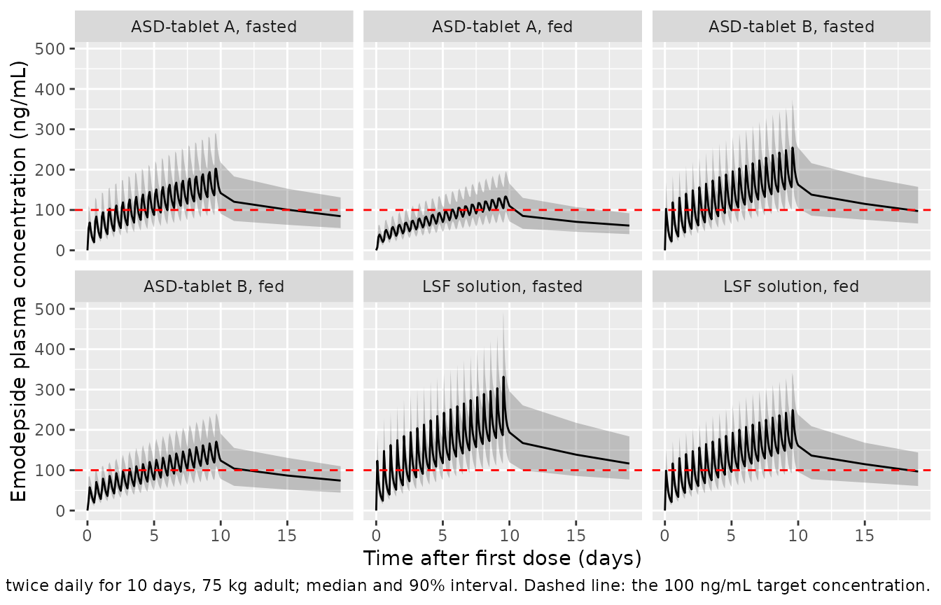
S3 Table reports stochastic-simulation medians (5th-95th percentiles) of the last-dose Cmax, Tmax, AUC from the first dose to infinity and the terminal half-life for 10 mg twice daily for 10 days in a 75 kg adult, for each formulation dosed fasted or fed. That regimen is reproduced here with 200 virtual subjects per arm.

set.seed(20220310)
rxode2::rxSetSeed(20220310)

n_per_arm <- 200L
arms <- tidyr::expand_grid(
  formulation = c("LSF solution", "ASD-tablet A", "ASD-tablet B"),
  food = c("fasted", "fed")
) |>
  mutate(
    arm = paste(formulation, food, sep = ", "),
    arm_index = dplyr::row_number()
  )

# 20 doses: 10 mg every 12 h from 0 to 228 h. The last-dose interval is
# densely sampled; the tail runs to 4,400 h (~10 half-lives after the last
# dose) so AUC to infinity is essentially observed. The tail is sampled
# every 4 days: ample for an 18-day half-life, and it keeps PKNCA's
# terminal-slope search fast.
dose_times <- seq(0, 228, by = 12)
obs_times <- sort(unique(c(
  seq(0, 228, by = 2),
  228 + c(0.25, 0.5, 0.75, 1, 1.25, 1.5, 1.75, 2, 2.5, 3, 3.5, 4, 5, 6, 8, 10, 12),
  seq(264, 4400, by = 96)
)))

make_arm <- function(arm_row, n) {
  ids <- (arm_row$arm_index - 1L) * n + seq_len(n)
  subj <- tibble(
    id = ids,
    arm = arm_row$arm,
    WT = 75,
    FED = as.integer(arm_row$food == "fed"),
    FORM_EMODEPSIDE_ASDA = as.integer(arm_row$formulation == "ASD-tablet A"),
    FORM_EMODEPSIDE_ASDB = as.integer(arm_row$formulation == "ASD-tablet B"),
    DOSE_EMODEPSIDE_MGKGD = 20 / 75,
    OCC = 0L
  )
  doses <- tidyr::crossing(subj, time = dose_times) |>
    mutate(amt = 10, evid = 1L, cmt = "depot", dvid = NA_integer_)
  obs <- tidyr::crossing(subj, time = obs_times) |>
    mutate(amt = NA_real_, evid = 0L, cmt = NA_character_, dvid = 1L)
  dplyr::bind_rows(doses, obs)
}

events_s3 <- dplyr::bind_rows(lapply(
  seq_len(nrow(arms)),
  function(i) make_arm(arms[i, ], n_per_arm)
)) |>
  dplyr::arrange(id, time, dplyr::desc(evid))
stopifnot(!anyDuplicated(unique(events_s3[, c("id", "time", "evid")])))

mod_pk <- readModelDb("Assmus_2022_emodepside")
sim_s3 <- rxode2::rxSolve(
  mod_pk,
  events = events_s3,
  keep = c("arm"),
  sigma = NA,
  returnType = "data.frame"
)
#> ℹ parameter labels from comments will be replaced by 'label()'
#> Warning: some etas defaulted to non-mu referenced, possible parsing error: etaiov_mtt_1, etaiov_mtt_2
#> as a work-around try putting the mu-referenced expression on a simple line

sim_s3 |>
  filter(time <= 480) |>
  group_by(arm, time) |>
  summarise(
    Q05 = quantile(Cc, 0.05),
    Q50 = median(Cc),
    Q95 = quantile(Cc, 0.95),
    .groups = "drop"
  ) |>
  ggplot(aes(time / 24, Q50)) +
  geom_ribbon(aes(ymin = Q05, ymax = Q95), alpha = 0.25) +
  geom_line() +
  geom_hline(yintercept = 100, linetype = "dashed", colour = "red") +
  facet_wrap(~arm, ncol = 3) +
  labs(
    x = "Time after first dose (days)",
    y = "Emodepside plasma concentration (ng/mL)",
    caption = paste(
      "10 mg twice daily for 10 days, 75 kg adult; median and 90% interval.",
      "Dashed line: the 100 ng/mL target concentration."
    )
  )

PKNCA computes Cmax and Tmax over the last dosing interval (228-240 h) and AUC and half-life over the whole profile from the first dose.

conc_s3 <- sim_s3 |>
  filter(!is.na(Cc)) |>
  select(id, time, Cc, arm)
conc_s3 <- dplyr::bind_rows(
  conc_s3,
  conc_s3 |> distinct(id, arm) |> mutate(time = 0, Cc = 0)
) |>
  distinct(id, arm, time, .keep_all = TRUE) |>
  arrange(id, arm, time)

dose_s3 <- events_s3 |>
  filter(evid == 1) |>
  select(id, time, amt, arm)

intervals_s3 <- data.frame(
  start = c(228, 0),
  end = c(240, Inf),
  cmax = c(TRUE, FALSE),
  tmax = c(TRUE, FALSE),
  aucinf.obs = c(FALSE, TRUE),
  half.life = c(FALSE, TRUE)
)

# One pk.nca() call per arm: a single call over all 1,200 subjects is slow
# (its run time grows faster than linearly with the number of groups).
nca_one_arm <- function(a) {
  res <- PKNCA::pk.nca(PKNCA::PKNCAdata(
    PKNCA::PKNCAconc(filter(conc_s3, arm == a), Cc ~ time | arm + id),
    PKNCA::PKNCAdose(filter(dose_s3, arm == a), amt ~ time | arm + id),
    intervals = intervals_s3
  ))
  as.data.frame(res)
}
# The half-life calculation over 0-Inf also reports the whole-profile Cmax
# and Tmax as dependencies; keep only the last-dose-interval values so the
# per-arm medians below are not pooled across the two intervals.
nca_s3 <- dplyr::bind_rows(lapply(unique(conc_s3$arm), nca_one_arm)) |>
  filter(!(PPTESTCD %in% c("cmax", "tmax") & start != 228))

# S3 Table medians. AUC converted from ug*h/mL to ng*h/mL; half-life from
# days to hours (18.4 days = 441.6 h, identical for every arm).
published_s3 <- tibble::tribble(
  ~arm,                     ~cmax, ~tmax, ~aucinf.obs, ~half.life,
  "LSF solution, fasted",   348,   1.11,  155000,      441.6,
  "LSF solution, fed",      245,   2.09,  117000,      441.6,
  "ASD-tablet A, fasted",   211,   3.09,  106000,      441.6,
  "ASD-tablet A, fed",      145,   5.67,   80000,      441.6,
  "ASD-tablet B, fasted",   258,   2.38,  124000,      441.6,
  "ASD-tablet B, fed",      179,   4.40,   94000,      441.6
)

cmp_s3 <- nlmixr2lib::ncaComparisonTable(
  simulated = nca_s3,
  reference = published_s3,
  by = "arm",
  units = c(
    cmax = "ng/mL", tmax = "h",
    aucinf.obs = "ng*h/mL", half.life = "h"
  ),
  tolerance_pct = 20
)
knitr::kable(
  cmp_s3,
  caption = paste(
    "Simulated (median of 200 subjects per arm) vs. S3 Table medians.",
    "* differs from the reference by >20%."
  )
)

Simulated (median of 200 subjects per arm) vs. S3 Table medians. * differs from the reference by >20%.
NCA parameter	arm	Reference	Simulated	% diff
Cmax (ng/mL)	LSF solution, fasted	348	344	-1.2%
Cmax (ng/mL)	LSF solution, fed	245	263	+7.5%
Cmax (ng/mL)	ASD-tablet A, fasted	211	210	-0.6%
Cmax (ng/mL)	ASD-tablet A, fed	145	140	-3.5%
Cmax (ng/mL)	ASD-tablet B, fasted	258	262	+1.6%
Cmax (ng/mL)	ASD-tablet B, fed	179	176	-1.8%
Tmax (h)	LSF solution, fasted	1.11	1	-9.9%
Tmax (h)	LSF solution, fed	2.09	2	-4.3%
Tmax (h)	ASD-tablet A, fasted	3.09	3	-2.9%
Tmax (h)	ASD-tablet A, fed	5.67	6	+5.8%
Tmax (h)	ASD-tablet B, fasted	2.38	2	-16.0%
Tmax (h)	ASD-tablet B, fed	4.4	4	-9.1%
AUC0-∞ (obs) (ng*h/mL)	LSF solution, fasted	155000	151000	-2.8%
AUC0-∞ (obs) (ng*h/mL)	LSF solution, fed	117000	118000	+1.1%
AUC0-∞ (obs) (ng*h/mL)	ASD-tablet A, fasted	106000	108000	+2.2%
AUC0-∞ (obs) (ng*h/mL)	ASD-tablet A, fed	80000	78600	-1.7%
AUC0-∞ (obs) (ng*h/mL)	ASD-tablet B, fasted	124000	124000	+0.3%
AUC0-∞ (obs) (ng*h/mL)	ASD-tablet B, fed	94000	93300	-0.7%
t½ (h)	LSF solution, fasted	442	459	+4.0%
t½ (h)	LSF solution, fed	442	462	+4.6%
t½ (h)	ASD-tablet A, fasted	442	453	+2.5%
t½ (h)	ASD-tablet A, fed	442	463	+4.8%
t½ (h)	ASD-tablet B, fasted	442	455	+3.0%
t½ (h)	ASD-tablet B, fed	442	471	+6.6%

Simulated Tmax is read off the sampling grid (0.25-1 h steps in the last-dose interval), whereas S3 Table reports the median over all dosing events, so its agreement is only to within one grid step and it is not gated. Cmax, AUC and half-life are.

# Median-based gate. Every arm shares the same disposition parameters, so a
# transcription error in CL, a volume, F or a formulation / food effect moves
# the corresponding medians by 20% or more. The observed differences are
# within +/- 8% (the largest, LSF fed Cmax, is +7.5% although its typical
# value matches S3 Table within 1%: it is sampling noise in a 200-subject
# median), so the 12% bound keeps headroom for a different cohort draw.
sim_medians <- nca_s3 |>
  filter(PPTESTCD %in% c("cmax", "aucinf.obs", "half.life")) |>
  group_by(arm, PPTESTCD) |>
  summarise(sim = median(PPORRES, na.rm = TRUE), .groups = "drop") |>
  left_join(
    published_s3 |>
      select(arm, cmax, aucinf.obs, half.life) |>
      pivot_longer(-arm, names_to = "PPTESTCD", values_to = "pub"),
    by = c("arm", "PPTESTCD")
  ) |>
  mutate(pct_diff = 100 * (sim - pub) / pub)
knitr::kable(sim_medians, digits = 1)

arm	PPTESTCD	sim	pub	pct_diff
ASD-tablet A, fasted	aucinf.obs	108317.5	106000.0	2.2
ASD-tablet A, fasted	cmax	209.7	211.0	-0.6
ASD-tablet A, fasted	half.life	452.5	441.6	2.5
ASD-tablet A, fed	aucinf.obs	78641.4	80000.0	-1.7
ASD-tablet A, fed	cmax	139.9	145.0	-3.5
ASD-tablet A, fed	half.life	462.9	441.6	4.8
ASD-tablet B, fasted	aucinf.obs	124409.1	124000.0	0.3
ASD-tablet B, fasted	cmax	262.2	258.0	1.6
ASD-tablet B, fasted	half.life	455.0	441.6	3.0
ASD-tablet B, fed	aucinf.obs	93346.5	94000.0	-0.7
ASD-tablet B, fed	cmax	175.8	179.0	-1.8
ASD-tablet B, fed	half.life	470.9	441.6	6.6
LSF solution, fasted	aucinf.obs	150682.1	155000.0	-2.8
LSF solution, fasted	cmax	344.0	348.0	-1.2
LSF solution, fasted	half.life	459.1	441.6	4.0
LSF solution, fed	aucinf.obs	118294.6	117000.0	1.1
LSF solution, fed	cmax	263.4	245.0	7.5
LSF solution, fed	half.life	461.9	441.6	4.6

stopifnot(
  all(abs(sim_medians$pct_diff[sim_medians$PPTESTCD == "cmax"]) < 12),
  all(abs(sim_medians$pct_diff[sim_medians$PPTESTCD == "aucinf.obs"]) < 12),
  all(abs(sim_medians$pct_diff[sim_medians$PPTESTCD == "half.life"]) < 15)
)

The venous-plasma-to-DBS scaling is a fixed ratio, so the DBS prediction is 0.618 times the plasma prediction at every time point:

positive <- sim_s3$Cc > 0
ratio <- sim_s3$Cb[positive] / sim_s3$Cc[positive]
stopifnot(all(abs(ratio - 0.618) < 1e-8))
range(ratio)
#> [1] 0.618 0.618

Dose-finding simulations: S4 Fig

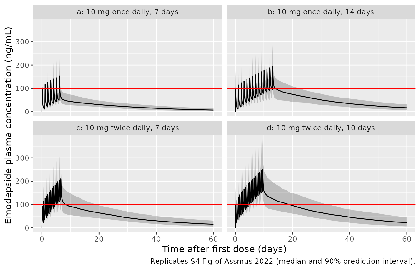
S4 Fig simulates ASD-tablet B, fasted, in a 75 kg adult for four candidate regimens and reports the median (5th-95th percentile) total time above the 100 ng/mL target. The same regimens are simulated here.

regimens <- tibble::tribble(
  ~regimen,                      ~interval, ~n_doses, ~daily_mg,
  "a: 10 mg once daily, 7 days",  24,        7,        10,
  "b: 10 mg once daily, 14 days", 24,        14,       10,
  "c: 10 mg twice daily, 7 days", 12,        14,       20,
  "d: 10 mg twice daily, 10 days", 12,       20,       20
) |>
  mutate(reg_index = dplyr::row_number())

grid_s4 <- seq(0, 60 * 24, by = 1)

make_regimen <- function(r, n) {
  ids <- 10000L + (r$reg_index - 1L) * n + seq_len(n)
  subj <- tibble(
    id = ids,
    regimen = r$regimen,
    WT = 75,
    FED = 0L,
    FORM_EMODEPSIDE_ASDA = 0L,
    FORM_EMODEPSIDE_ASDB = 1L,
    DOSE_EMODEPSIDE_MGKGD = r$daily_mg / 75,
    OCC = 0L
  )
  doses <- tidyr::crossing(
    subj,
    time = seq(0, by = r$interval, length.out = r$n_doses)
  ) |>
    mutate(amt = 10, evid = 1L, cmt = "depot", dvid = NA_integer_)
  obs <- tidyr::crossing(subj, time = grid_s4) |>
    mutate(amt = NA_real_, evid = 0L, cmt = NA_character_, dvid = 1L)
  dplyr::bind_rows(doses, obs)
}

events_s4 <- dplyr::bind_rows(lapply(
  seq_len(nrow(regimens)),
  function(i) make_regimen(regimens[i, ], n_per_arm)
)) |>
  dplyr::arrange(id, time, dplyr::desc(evid))
stopifnot(!anyDuplicated(unique(events_s4[, c("id", "time", "evid")])))

sim_s4 <- rxode2::rxSolve(
  mod_pk,
  events = events_s4,
  keep = c("regimen"),
  sigma = NA,
  returnType = "data.frame"
)

time_above <- sim_s4 |>
  group_by(regimen, id) |>
  summarise(days_above = sum(Cc > 100) / 24, .groups = "drop") |>
  group_by(regimen) |>
  summarise(
    median = median(days_above),
    p05 = quantile(days_above, 0.05),
    p95 = quantile(days_above, 0.95),
    .groups = "drop"
  ) |>
  mutate(
    published_median = c(0.9, 3.6, 5.4, 15.9),
    published_interval = c("0.0-2.0", "1.0-16.5", "1.6-17.2", "3.9-30.1")
  )
time_above |>
  dplyr::rename(
    "Regimen" = regimen,
    "Simulated median (days)" = median,
    "Simulated 5th pct" = p05,
    "Simulated 95th pct" = p95,
    "S4 Fig median (days)" = published_median,
    "S4 Fig 5th-95th pct" = published_interval
  ) |>
  knitr::kable(digits = 1, caption = "Total time above 100 ng/mL, ASD-tablet B fasted, 75 kg.")

Total time above 100 ng/mL, ASD-tablet B fasted, 75 kg.
Regimen	Simulated median (days)	Simulated 5th pct	Simulated 95th pct	S4 Fig median (days)	S4 Fig 5th-95th pct
a: 10 mg once daily, 7 days	0.9	0.1	1.8	0.9	0.0-2.0
b: 10 mg once daily, 14 days	4.4	1.0	17.0	3.6	1.0-16.5
c: 10 mg twice daily, 7 days	5.6	1.8	17.3	5.4	1.6-17.2
d: 10 mg twice daily, 10 days	15.8	4.7	30.5	15.9	3.9-30.1

# Gate on the medians of the two regimens that were carried forward, whose
# published values sit well away from the 0-day floor. The tolerance is
# absolute (days) because a CL or F transcription error shifts these
# medians by several days.
stopifnot(
  abs(time_above$median[3] - 5.4) < 1.5,
  abs(time_above$median[4] - 15.9) < 3
)

sim_s4 |>
  group_by(regimen, time) |>
  summarise(
    Q05 = quantile(Cc, 0.05),
    Q50 = median(Cc),
    Q95 = quantile(Cc, 0.95),
    .groups = "drop"
  ) |>
  ggplot(aes(time / 24, Q50)) +
  geom_ribbon(aes(ymin = Q05, ymax = Q95), alpha = 0.25) +
  geom_line() +
  geom_hline(yintercept = 100, colour = "red") +
  facet_wrap(~regimen) +
  labs(
    x = "Time after first dose (days)",
    y = "Emodepside plasma concentration (ng/mL)",
    caption = "Replicates S4 Fig of Assmus 2022 (median and 90% prediction interval)."
  )

Exposure-adverse event models

The four logistic regressions are static: each maps one individual Cmax to an event probability. The Results give worked probabilities at 300, 400 and 500 ng/mL for three of them, which the packaged models reproduce.

er_models <- c(
  "TEAE of interest" = "Assmus_2022_emodepside_teae_interest",
  "Eye disorder" = "Assmus_2022_emodepside_eye_disorder",
  "Nervous system disorder" = "Assmus_2022_emodepside_nervous_system_disorder",
  "Any drug-related TEAE" = "Assmus_2022_emodepside_teae_drug_related"
)
cmax_grid <- data.frame(id = seq_len(151), time = 0, CMAX = seq(0, 750, by = 5))

er_pred <- dplyr::bind_rows(lapply(names(er_models), function(nm) {
  m <- readModelDb(er_models[[nm]])
  out <- rxode2::rxSolve(m, events = cmax_grid, omega = NA, sigma = NA,
                         returnType = "data.frame")
  prob_col <- grep("^prob_", names(out), value = TRUE)
  data.frame(endpoint = nm, CMAX = cmax_grid$CMAX, prob = out[[prob_col]])
}))

published_prob <- tibble::tribble(
  ~endpoint,                 ~CMAX, ~published,
  "TEAE of interest",        300,   0.36,
  "TEAE of interest",        400,   0.55,
  "TEAE of interest",        500,   0.73,
  "Eye disorder",            300,   0.263,
  "Eye disorder",            400,   0.456,
  "Eye disorder",            500,   0.66,
  "Nervous system disorder", 300,   0.211,
  "Nervous system disorder", 400,   0.333,
  "Nervous system disorder", 500,   0.48
)
er_check <- published_prob |>
  left_join(er_pred, by = c("endpoint", "CMAX")) |>
  mutate(diff_pct_points = 100 * (prob - published))
knitr::kable(er_check, digits = 3,
             caption = "Predicted vs. published probabilities (Results, 'Exposure-adverse events analysis').")

Predicted vs. published probabilities (Results, ‘Exposure-adverse events analysis’).
endpoint	CMAX	published	prob	diff_pct_points
TEAE of interest	300	0.360	0.364	0.355
TEAE of interest	400	0.550	0.552	0.231
TEAE of interest	500	0.730	0.727	-0.289
Eye disorder	300	0.263	0.261	-0.185
Eye disorder	400	0.456	0.453	-0.336
Eye disorder	500	0.660	0.659	-0.074
Nervous system disorder	300	0.211	0.212	0.149
Nervous system disorder	400	0.333	0.336	0.326
Nervous system disorder	500	0.480	0.488	0.750

# Deterministic: the published values were computed from the same
# coefficients, rounded. The residual differences are rounding only.
stopifnot(all(abs(er_check$diff_pct_points) < 1.5))

ggplot(er_pred, aes(CMAX, prob, colour = endpoint)) +
  geom_line() +
  geom_hline(yintercept = 0.5, linetype = "dotted", colour = "red") +
  geom_point(data = published_prob, aes(y = published), size = 2) +
  labs(
    x = "Individual maximum plasma concentration (ng/mL)",
    y = "Probability of drug-related TEAE",
    colour = NULL,
    caption = paste(
      "Lines: packaged models. Points: worked values from the Results.",
      "Dotted line: the 50% tolerability threshold (compare Fig 3, lower panels)."
    )
  ) +
  theme(legend.position = "bottom")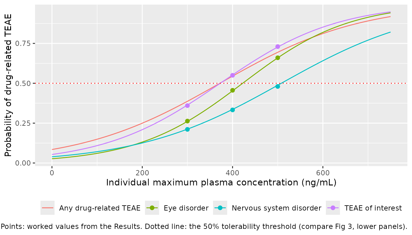

Chaining the two layers: the per-subject Cmax from the S3 simulation above (last-dose peak of 10 mg twice daily for 10 days, 75 kg) feeds the TEAE-of-interest model. The paper’s regimen choice required the median probability to stay below 50%.

cmax_subj <- nca_s3 |>
  filter(PPTESTCD == "cmax") |>
  select(id, arm, CMAX = PPORRES) |>
  mutate(time = 0)
chain <- rxode2::rxSolve(
  readModelDb("Assmus_2022_emodepside_teae_interest"),
  events = cmax_subj |> select(id, time, CMAX),
  omega = NA, sigma = NA, returnType = "data.frame"
) |>
  select(id, prob_teae_interest) |>
  left_join(cmax_subj |> select(id, arm), by = "id")
chain |>
  group_by(arm) |>
  summarise(
    median_prob = median(prob_teae_interest),
    p05 = quantile(prob_teae_interest, 0.05),
    p95 = quantile(prob_teae_interest, 0.95),
    .groups = "drop"
  ) |>
  knitr::kable(digits = 3,
               caption = "Predicted probability of a drug-related TEAE of interest, 10 mg twice daily for 10 days, 75 kg.")

Predicted probability of a drug-related TEAE of interest, 10 mg twice daily for 10 days, 75 kg.
arm	median_prob	p05	p95
ASD-tablet A, fasted	0.222	0.144	0.378
ASD-tablet A, fed	0.143	0.108	0.209
ASD-tablet B, fasted	0.299	0.180	0.531
ASD-tablet B, fed	0.180	0.122	0.278
LSF solution, fasted	0.445	0.251	0.729
LSF solution, fed	0.301	0.171	0.455

Assumptions and deviations

Peripheral compartment numbering. The S1 Code labels the deep peripheral compartment (Q = 8.45 L/h, V = 647 L) as compartment 1 and the shallow one (Q = 4.6 L/h, V = 44.4 L) as compartment 2, while Table 3 and the Discussion number them the other way round. The Q-V pairings and the IIV assignments agree between the two sources (the Table 3 %CVs reproduce exactly from the S1 Code variances on the matching parameters), so only the labels differ. The model follows Table 3: peripheral1 is the shallow compartment.
ASD-tablet B effect on MTT. The Results prose says tablets A and B lengthened absorption by “243% and 114%”; Table 3 and the S1 Code (THETA(13) = 1.24) give 124% for tablet B. The model uses 124%; the 114% in the prose repeats the food effect on MTT.
Inter-occasion variability is carried only for the multiple ascending dose study, as in the S1 Code (IF(STUDY_ID.EQ.2)). Supply OCC = 1 for days 0-6 of dosing and OCC = 2 from day 7 to reproduce it; every other record takes OCC = 0. The simulations in this article use OCC = 0. The paper does not say whether its S3 Table and dose-finding simulations included IOV; with ~75% shrinkage its influence on the medians compared here is small.
Shrinkage text. The Results quote an eta shrinkage for ‘Vp1/F’, which carries no IIV in the final model; it presumably refers to Vp2/F. This does not affect any value in the model.
Dose covariate. DOSE_EMODEPSIDE_MGKGD is the total daily dose divided by body weight, centred at 0.08 mg/kg/day in the S1 Code. It must be set for every subject, including single-dose ones (the single dose divided by weight).
Residual error in the S3 and S4 comparisons. The published tables and figure summarise individual predictions; residual error is switched off (sigma = NA) here. Cc is the individual prediction in either case.
Logistic models. The four models have no random effect and no residual error (Bernoulli likelihood, fitted in R). The fixed additive residual SD of 0.001 on each probability is a placeholder so rxode2 has an error model and is not a published quantity. Only the Cmax models, selected by the authors over AUC to infinity, daily dose and cumulative dose, are packaged. The Results prose gives the nervous-system odds increase as 0.62% per ng/mL; S6 Table prints 0.63% and the log-odds 0.0063 used here.
CMAX definition. The paper derived Cmax per subject from the final PK model; for the multiple ascending dose study this is the peak over the 10-day regimen. Most events occurred 1-3 h after a dose, shortly after Tmax.
Body-weight-based phase II regimens (Fig 4 and Fig 5) are given only as a figure; their dose bands were not transcribed and they are not reproduced here.
Erratum check. No correction notice for this article was found on the PLoS landing page or in Europe PMC as of 2026-09-30.