Avadomide (Cheng 2021) • nlmixr2lib

Model and source

Citation: Cheng Y, Chen J, Pourdehnad M, Zhou S, Li Y. Population Pharmacokinetics of CC-122. Clin Pharmacol. 2021;13:61-71. doi:10.2147/CPAA.S310604.
Article: https://doi.org/10.2147/CPAA.S310604 (open access)

Avadomide (CC-122) is an oral cereblon-modulating agent. The packaged model Cheng_2021_avadomide is the final population PK model of Cheng 2021: a two-compartment model with first-order absorption after an absorption lag time (ALAG = 0.246 h) and first-order elimination. The peripheral volume was fixed at 10 L. Apparent clearance depends on creatinine clearance (linear, centred at 94.42 mL/min) and on four tumor types (DLBCL, PCNSL, other solid tumor and multiple myeloma); the apparent central volume depends on body weight (linear, centred at 74.5 kg), female sex and seven tumor types. Healthy male subjects are the reference. Residual error is additive on log-transformed concentrations, encoded as lnorm().

Population

Cheng 2021 pooled 298 subjects from three studies (Table 1):

CC-122-CP-002 Part 1 (n = 30): single ascending oral doses in healthy adults.
CC-122-CP-005 (n = 48): single oral dose in subjects with mild, moderate or severe renal impairment and matched healthy subjects.
CC-122-ST-001 (NCT01421524, n = 220): phase 1a/b dose finding in patients with advanced solid tumors, non-Hodgkin lymphoma (NHL) or multiple myeloma (MM).

Median (range) age was 59.5 (20-91) years, body weight 74.5 (39.8-159.0) kg and creatinine clearance 94.4 (9.0-321.2) mL/min; 37.9% were female. Tumor types were healthy (no tumor) 78 (26.2%), DLBCL 60 (20.1%), GBM 44 (14.8%), NHL 30 (10.1%), MM 29 (9.7%), HCC 27 (9.1%), other solid tumor 19 (6.4%), brain cancer 6 (2.0%) and primary CNS lymphoma (PCNSL) 5 (1.7%). Doses ranged from 0.5 to 15 mg. Race and region were not reported.

The same information is available programmatically via readModelDb("Cheng_2021_avadomide")()$population.

Source trace

Every ini() value carries an in-file comment in inst/modeldb/specificDrugs/Cheng_2021_avadomide.R. The table below collects them.

Equation / parameter	Value	Source location
`lka` (Ka)	log(4.14) 1/h	Table 2, TVKa
`ltlag` (ALAG)	log(0.246) h	Table 2, TVALAG
`lcl` (CL/F)	log(3.63) L/h	Table 2, TVCL/F
`lvc` (V2/F)	log(36.2) L	Table 2, TVV2/F
`lq` (Q/F)	log(1.38) L/h	Table 2, TVQ/F
`lvp` (V3/F)	fixed(log(10)) L	Table 2, TVV3/F ‘10 Fix’; Results, Structural model
`e_crcl_cl`	0.007 per mL/min	Table 2 and footnote b
`e_tumtp_dlbcl_cl`, `e_tumtp_pcnsl_cl`, `e_tumtp_other_cl`, `e_tumtp_myelo_cl`	-0.647, -0.692, -0.364, 0.309	Table 2 and footnote b
`e_wt_vc`	0.009 per kg	Table 2 and footnote c
`e_sexf_vc`	-0.179	Table 2 and footnote c (‘(1 - 0.179) if female’)
`e_tumtp_*_vc` (DLBCL, PCNSL, NHL, HCC, GBM, MM, brain cancer)	0.476, 0.846, 0.344, 0.521, 0.480, 0.682, 0.415	Table 2 and footnote c
`etalcl`, `etalvc`, `etalka`, `etalq`	0.2725, 0.0681, 2.0506, 0.9624	Table 2 CV% squared (52.2%, 26.1%, 143.2%, 98.1%)
`expSd`	0.3033	Table 2, sigma^2 (log additive) = 0.092
CL/F equation	`3.63 * (1 + 0.007 * (CLcr - 94.42)) * prod(1 + theta_k * Z_k)`	Table 2 footnote b; Methods Eqs. 1 and 3
V2/F equation	`36.2 * (1 + 0.009 * (BW - 74.5)) * (1 - 0.179)^female * prod(1 + theta_k * Z_k)`	Table 2 footnote c
Structure: `d/dt(depot)`, `d/dt(central)`, `d/dt(peripheral1)`, `alag(depot)`	n/a	Figure 3; Results, Structural model
Residual error `Cc ~ lnorm(expSd)`	n/a	Methods: additive error after log-transforming predictions

Typical-value covariate effects (Figure 4)

Figure 4 is a forest plot of the covariate effects on CL/F and V2/F. The Results text reports the numbers behind it, which the model’s covariate factors can be set against directly.

mod <- readModelDb("Cheng_2021_avadomide")
theta <- rxode2::rxode(mod)$theta
#> ℹ parameter labels from comments will be replaced by 'label()'

cl_factor <- tibble::tribble(
  ~category,           ~model,                               ~paper_pct,
  "DLBCL",             1 + theta[["e_tumtp_dlbcl_cl"]],      34.8,
  "PCNSL",             1 + theta[["e_tumtp_pcnsl_cl"]],      30.3,
  "Other solid tumor", 1 + theta[["e_tumtp_other_cl"]],      73.7,
  "MM",                1 + theta[["e_tumtp_myelo_cl"]],      120.0,
  "NHL",               1,                                    89.3,
  "HCC",               1,                                    109.2,
  "GBM",               1,                                    107.9,
  "Brain cancer",      1,                                    131.6
) |>
  dplyr::mutate(model_pct = 100 * model)

cl_factor |>
  dplyr::select(category, model_pct, paper_pct) |>
  dplyr::rename(
    "Tumor type" = category,
    "Model CL/F, % of healthy" = model_pct,
    "Results text, % of healthy" = paper_pct
  ) |>
  knitr::kable(digits = 1, caption = "Typical CL/F by tumor type relative to healthy subjects.")

Typical CL/F by tumor type relative to healthy subjects.
Tumor type	Model CL/F, % of healthy	Results text, % of healthy
DLBCL	35.3	34.8
PCNSL	30.8	30.3
Other solid tumor	63.6	73.7
MM	130.9	120.0
NHL	100.0	89.3
HCC	100.0	109.2
GBM	100.0	107.9
Brain cancer	100.0	131.6


# Structural gate: the two large, precisely estimated CL/F effects must
# reproduce the Results text to within 2 percentage points. A sign or
# transcription error in either coefficient moves the factor by tens of points.
stopifnot(
  abs(cl_factor$model_pct[cl_factor$category == "DLBCL"] - 34.8) < 2,
  abs(cl_factor$model_pct[cl_factor$category == "PCNSL"] - 30.3) < 2
)

The DLBCL and PCNSL factors agree with the text. The remaining percentages in the text do not come from the Table 2 coefficients: for NHL, HCC, GBM and brain cancer the text reports 89.3-131.6% of healthy CL/F and then states that these effects were fixed to 0 in the model, so the text values describe individual estimates rather than the model. The same holds for other solid tumor (73.7% in the text, 63.6% from the coefficient) and MM (120.0% versus 130.9%). Figure 4 plots medians of individual estimates, so it is a descriptive summary and not a readout of Table 2.

vc_factor <- tibble::tribble(
  ~category,      ~model,
  "DLBCL",        1 + theta[["e_tumtp_dlbcl_vc"]],
  "PCNSL",        1 + theta[["e_tumtp_pcnsl_vc"]],
  "NHL",          1 + theta[["e_tumtp_nhl_vc"]],
  "HCC",          1 + theta[["e_tumtp_hcc_vc"]],
  "GBM",          1 + theta[["e_tumtp_glio_vc"]],
  "MM",           1 + theta[["e_tumtp_myelo_vc"]],
  "Brain cancer", 1 + theta[["e_tumtp_brain_vc"]],
  "Female",       1 + theta[["e_sexf_vc"]]
)
vc_factor |>
  dplyr::mutate(model = 100 * model) |>
  dplyr::rename("Category" = category, "Model V2/F, % of reference" = model) |>
  knitr::kable(digits = 1, caption = "Typical V2/F relative to healthy male subjects.")

Typical V2/F relative to healthy male subjects.
Category	Model V2/F, % of reference
DLBCL	147.6
PCNSL	184.6
NHL	134.4
HCC	152.1
GBM	148.0
MM	168.2
Brain cancer	141.5
Female	82.1

The text reports V2/F 3.3% to 57.8% higher in cancer patients and 26.8% higher in males. The coefficients give 34.4% to 84.6% higher V2/F by tumor type and 1 / (1 - 0.179) = 21.8% higher in males. These are again individual-estimate summaries (Figure 4B) and are not expected to match the coefficients.

Virtual cohort

The observed data are not public. The cohorts below approximate the demographics of each study in Table 1. Body weight and creatinine clearance are drawn log-normally around each study’s median and truncated to its range. ST-001 tumor types are drawn with the Table 1 counts (60 DLBCL, 5 PCNSL, 19 other solid tumor, 30 NHL, 27 HCC, 44 GBM, 29 MM, 6 brain cancer). Every subject gets a single 3 mg oral dose: the dose Li 2020 used in the renal impairment study (CP-005) and within the 0.5-15 mg range of the pooled data.

set.seed(2021)

rtrunc_lnorm <- function(n, median, sdlog, lo, hi) {
  pmin(pmax(median * exp(rnorm(n, 0, sdlog)), lo), hi)
}

tumor_levels <- c(
  "DLBCL", "PCNSL", "Other solid tumor", "NHL", "HCC", "GBM", "MM", "Brain cancer"
)
tumor_counts <- c(60, 5, 19, 30, 27, 44, 29, 6)

make_cohort <- function(n, study, wt_med, wt_lo, wt_hi, crcl_med, crcl_sd,
                        crcl_lo, crcl_hi, pct_female, tumor, id_offset) {
  tibble::tibble(
    id = id_offset + seq_len(n),
    study = study,
    WT = rtrunc_lnorm(n, wt_med, 0.2, wt_lo, wt_hi),
    CRCL = rtrunc_lnorm(n, crcl_med, crcl_sd, crcl_lo, crcl_hi),
    SEXF = rbinom(n, 1, pct_female / 100),
    tumor = tumor
  )
}

subjects <- dplyr::bind_rows(
  make_cohort(100, "CP-002", 75.8, 52.9, 95.0, 107.0, 0.2, 76.3, 171.0, 16.7,
              "Healthy", id_offset = 0L),
  make_cohort(100, "CP-005", 79.1, 57.7, 126.0, 90.6, 0.6, 9.0, 152.0, 43.7,
              "Healthy", id_offset = 100L),
  make_cohort(200, "ST-001", 73.0, 39.8, 159.0, 92.1, 0.3, 35.3, 321.2, 39.5,
              sample(rep(tumor_levels, tumor_counts), 200), id_offset = 200L)
) |>
  dplyr::mutate(
    TUMTP_DLBCL = as.integer(tumor == "DLBCL"),
    TUMTP_PCNSL = as.integer(tumor == "PCNSL"),
    TUMTP_OTHER = as.integer(tumor == "Other solid tumor"),
    TUMTP_NHL = as.integer(tumor == "NHL"),
    TUMTP_HCC = as.integer(tumor == "HCC"),
    TUMTP_GLIO = as.integer(tumor == "GBM"),
    TUMTP_MYELO = as.integer(tumor == "MM"),
    TUMTP_BRAIN = as.integer(tumor == "Brain cancer")
  )
stopifnot(!anyDuplicated(subjects$id))

obs_times <- c(0, 0.25, 0.5, 0.75, 1, 1.5, 2, 3, 4, 6, 8, 12, 24, 36, 48, 72)
dose_amt <- 3

events <- dplyr::bind_rows(
  subjects |> dplyr::mutate(time = 0, evid = 1L, amt = dose_amt, cmt = "depot"),
  subjects |>
    tidyr::crossing(time = obs_times) |>
    dplyr::mutate(evid = 0L, amt = 0, cmt = "central")
) |>
  dplyr::arrange(id, time, dplyr::desc(evid))

Simulation

keep_cols <- c("study", "tumor", "CRCL", "WT", "SEXF")
sim <- rxode2::rxSolve(mod, events = events, keep = keep_cols) |>
  as.data.frame()
#> ℹ parameter labels from comments will be replaced by 'label()'

mod_typical <- rxode2::zeroRe(mod)
#> ℹ parameter labels from comments will be replaced by 'label()'
sim_typical <- rxode2::rxSolve(mod_typical, events = events, keep = keep_cols) |>
  as.data.frame()
#> ℹ omega/sigma items treated as zero: 'etalcl', 'etalvc', 'etalka', 'etalq'
#> Warning: multi-subject simulation without without 'omega'

Replicate published figures

Figure 2: dose-normalized profiles by study

sim |>
  dplyr::filter(!is.na(Cc)) |>
  dplyr::mutate(cn = Cc / dose_amt) |>
  dplyr::group_by(study, time) |>
  dplyr::summarise(
    Q05 = quantile(cn, 0.05), Q50 = median(cn), Q95 = quantile(cn, 0.95),
    .groups = "drop"
  ) |>
  ggplot(aes(time, Q50, colour = study, fill = study)) +
  geom_ribbon(aes(ymin = Q05, ymax = Q95), alpha = 0.15, colour = NA) +
  geom_line(linewidth = 0.8) +
  labs(
    x = "Time after dose (h)", y = "Concentration / dose (ng/mL/mg)",
    colour = "Study", fill = "Study",
    title = "Simulated dose-normalized CC-122 profiles by study (median, 5th-95th)",
    caption = "Compare with Figure 2 of Cheng 2021 (individual observed profiles)."
  )

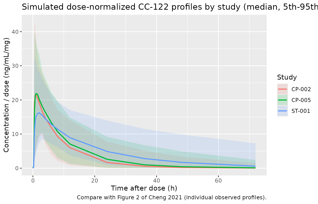
Figure 2 of the paper shows most dose-normalized peaks between about 20 and 60 ng/mL/mg, with the widest spread in ST-001. In the simulation the typical healthy peak is about 23 ng/mL/mg (Cmax / 3 mg in the NCA table below). ST-001 patients have lower median peaks because most tumor types raise V2/F by 34-85%, and they decline more slowly because DLBCL and PCNSL cut CL/F by about two-thirds. CP-005 declines more slowly than CP-002 because of its renally impaired subjects. The figure shows individual observed profiles, so the comparison is qualitative.

Figure 5: VPC of log concentration

# Add the log-additive residual error explicitly (sigma^2 = 0.092) so the
# percentiles are those of simulated observations, as in a VPC.
exp_sd <- theta[["expSd"]]
sim |>
  dplyr::filter(!is.na(Cc), time > 0) |>
  dplyr::mutate(log_obs = log(Cc) + rnorm(dplyr::n(), 0, exp_sd)) |>
  dplyr::group_by(time) |>
  dplyr::summarise(
    Q05 = quantile(log_obs, 0.05), Q50 = median(log_obs),
    Q95 = quantile(log_obs, 0.95), .groups = "drop"
  ) |>
  ggplot(aes(time, Q50)) +
  geom_ribbon(aes(ymin = Q05, ymax = Q95), alpha = 0.25, fill = "steelblue") +
  geom_line(colour = "firebrick", linewidth = 0.8) +
  labs(
    x = "Time after dose (hours)", y = "Log(CC-122) (ng/mL)",
    title = "Simulated 5th, 50th and 95th percentiles, pooled cohort, 3 mg",
    caption = "Compare with Figure 5 of Cheng 2021 (doses pooled, 0.5-15 mg)."
  )

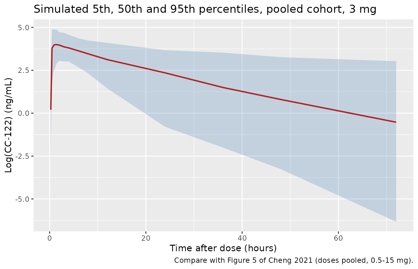
Figure 5 pools every dose level in the dataset, so the simulated 3 mg percentiles are a shape comparison only. Read by eye, the observed median in Figure 5 falls by about 1.7 log units between 24 and 48 h, which corresponds to a half-life of about 10 h. The typical healthy subject in the model has a terminal half-life of the same size (computed below).

PKNCA validation

sim_nca <- sim |>
  dplyr::filter(!is.na(Cc)) |>
  dplyr::select(id, time, Cc, study)
sim_nca <- dplyr::bind_rows(
  sim_nca,
  sim_nca |> dplyr::distinct(id, study) |> dplyr::mutate(time = 0, Cc = 0)
) |>
  dplyr::distinct(id, study, time, .keep_all = TRUE) |>
  dplyr::arrange(id, study, time)

dose_df <- events |>
  dplyr::filter(evid == 1) |>
  dplyr::select(id, time, amt, study)

conc_obj <- PKNCA::PKNCAconc(sim_nca, Cc ~ time | study + id)
dose_obj <- PKNCA::PKNCAdose(dose_df, amt ~ time | study + id)
intervals <- data.frame(
  start = 0, end = Inf,
  cmax = TRUE, tmax = TRUE, aucinf.obs = TRUE, half.life = TRUE
)
nca_res <- PKNCA::pk.nca(PKNCA::PKNCAdata(conc_obj, dose_obj, intervals = intervals))

nca_summary <- as.data.frame(nca_res$result) |>
  dplyr::filter(PPTESTCD %in% c("cmax", "tmax", "aucinf.obs", "half.life")) |>
  dplyr::group_by(study, PPTESTCD) |>
  dplyr::summarise(median = median(PPORRES, na.rm = TRUE), .groups = "drop") |>
  tidyr::pivot_wider(names_from = PPTESTCD, values_from = median)

nca_summary |>
  dplyr::rename(
    "Study" = study,
    "Cmax (ng/mL)" = cmax,
    "Tmax (h)" = tmax,
    "AUC0-inf (ng*h/mL)" = aucinf.obs,
    "t1/2 (h)" = half.life
  ) |>
  knitr::kable(digits = 2, caption = "Median simulated NCA after a single 3 mg dose.")

Median simulated NCA after a single 3 mg dose.
Study	AUC0-inf (ng*h/mL)	Cmax (ng/mL)	t1/2 (h)	Tmax (h)
CP-002	634.52	70.00	10.68	1.0
CP-005	791.28	68.26	11.30	1.0
ST-001	1030.74	53.65	15.96	1.5

Comparison against published NCA

The Introduction of Cheng 2021 summarises the single-dose NCA in healthy adults (3 to 15 mg): Tmax approximately 1 h and terminal half-life 7.6-8.9 h. The healthy single-ascending-dose cohort (CP-002) is the matching simulated group.

published <- tibble::tibble(study = "CP-002", tmax = 1)
cmp <- nlmixr2lib::ncaComparisonTable(
  simulated = nca_res,
  reference = published,
  by = "study",
  params = "tmax",
  units = c(tmax = "h"),
  tolerance_pct = 20
)
knitr::kable(cmp, caption = "Simulated vs. published Tmax (CP-002, healthy). * differs by >20%.")

Simulated vs. published Tmax (CP-002, healthy). * differs by >20%.
NCA parameter	study	Reference	Simulated	% diff
Tmax (h)	CP-002	1	1	+0.0%


hl_cp002 <- nca_summary$half.life[nca_summary$study == "CP-002"]
tmax_cp002 <- nca_summary$tmax[nca_summary$study == "CP-002"]

# Typical healthy reference subject: terminal (beta) half-life from the
# micro-constants (CLcr 94.42 mL/min, 74.5 kg, male).
k10 <- exp(theta[["lcl"]]) / exp(theta[["lvc"]])
k12 <- exp(theta[["lq"]]) / exp(theta[["lvc"]])
k21 <- exp(theta[["lq"]]) / exp(theta[["lvp"]])
beta <- ((k10 + k12 + k21) - sqrt((k10 + k12 + k21)^2 - 4 * k10 * k21)) / 2
hl_typical <- log(2) / beta

tibble::tibble(
  Quantity = c(
    "Median simulated t1/2, CP-002 (h)",
    "Typical-subject terminal t1/2 (h)",
    "Published t1/2 range, healthy (h)"
  ),
  Value = c(
    sprintf("%.1f", hl_cp002), sprintf("%.1f", hl_typical), "7.6-8.9"
  )
) |>
  knitr::kable(caption = "Terminal half-life.")

Terminal half-life.
Quantity	Value
Median simulated t1/2, CP-002 (h)	10.7
Typical-subject terminal t1/2 (h)	10.6
Published t1/2 range, healthy (h)	7.6-8.9


# Gates on medians of 100 simulated subjects. Tmax: lag 0.246 h plus
# Ka = 4.14 1/h puts the typical peak near 1 h; a mis-transcribed lag or Ka
# moves it by more than 0.5 h. Half-life: the typical value is ~10 h, and a
# broken Q/F or V3/F moves it by a factor of 2 or more.
stopifnot(
  abs(tmax_cp002 - 1) < 0.5,
  hl_typical > 7, hl_typical < 13,
  hl_cp002 > 6, hl_cp002 < 14
)

Simulated Tmax matches the published value. The model’s terminal half-life is longer than the published 7.6-8.9 h range. That range comes from a dense-sampling NCA of healthy adults in a separate report cited by the paper; the popPK model fixed V3/F at 10 L and estimated Q/F with a 49.9% RSE and a 98.1% CV, so its terminal phase is not tightly identified, and the difference is recorded here rather than adjusted.

Closed-form AUC check

For a linear model the typical-value AUC0-inf after an oral dose is Dose / (CL/F). This check runs on the zero-random-effect solve.

cl_typ <- sim_typical |>
  dplyr::distinct(id, .keep_all = TRUE) |>
  dplyr::select(id, study, cl)

conc_typ <- sim_typical |>
  dplyr::filter(!is.na(Cc)) |>
  dplyr::select(id, time, Cc, study)
conc_typ <- dplyr::bind_rows(
  conc_typ,
  conc_typ |> dplyr::distinct(id, study) |> dplyr::mutate(time = 0, Cc = 0)
) |>
  dplyr::distinct(id, study, time, .keep_all = TRUE) |>
  dplyr::arrange(id, time)

nca_typ <- PKNCA::pk.nca(PKNCA::PKNCAdata(
  PKNCA::PKNCAconc(conc_typ, Cc ~ time | study + id),
  PKNCA::PKNCAdose(dose_df, amt ~ time | study + id),
  intervals = data.frame(start = 0, end = Inf, aucinf.obs = TRUE)
))

auc_chk <- as.data.frame(nca_typ$result) |>
  dplyr::filter(PPTESTCD == "aucinf.obs") |>
  dplyr::select(id, study, auc = PPORRES) |>
  dplyr::left_join(cl_typ, by = c("id", "study")) |>
  dplyr::mutate(
    auc_closed = dose_amt * 1000 / cl,
    pct_diff = 100 * (auc / auc_closed - 1)
  )

auc_chk |>
  dplyr::group_by(study) |>
  dplyr::summarise(
    median_pct_diff = median(pct_diff),
    max_abs_pct_diff = max(abs(pct_diff)),
    .groups = "drop"
  ) |>
  dplyr::rename(
    "Study" = study,
    "Median % difference" = median_pct_diff,
    "Max |% difference|" = max_abs_pct_diff
  ) |>
  knitr::kable(digits = 2, caption = "PKNCA AUC0-inf vs Dose / (CL/F), typical values.")

PKNCA AUC0-inf vs Dose / (CL/F), typical values.
Study	Median % difference	Max \|% difference\|
CP-002	0.33	0.43
CP-005	0.31	0.42
ST-001	0.14	0.41


# Trapezoidal AUC over a 72 h grid plus log-linear extrapolation differs from
# the exact integral by a few percent; a wrong CL/F, dose or unit moves it by
# tens of percent.
stopifnot(
  abs(median(auc_chk$pct_diff)) < 5,
  quantile(abs(auc_chk$pct_diff), 0.9) < 10
)

Renal function

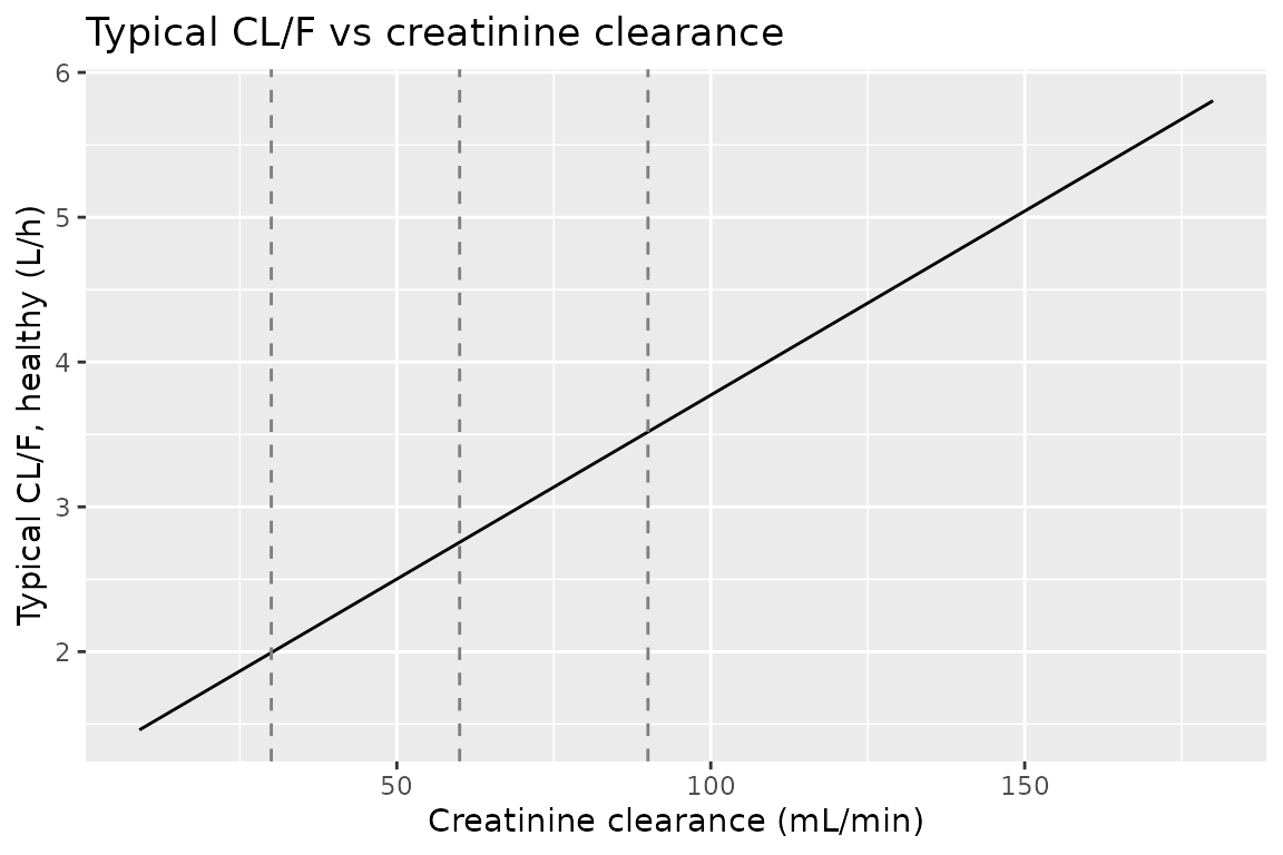
Cheng 2021 identified creatinine clearance as the covariate supporting dose adjustment in renal impairment. Because the effect is linear, typical CL/F falls to 40% of the reference at the lowest observed CLcr (9 mL/min).

crcl_grid <- tibble::tibble(CRCL = seq(9, 180, by = 1)) |>
  dplyr::mutate(
    cl = exp(theta[["lcl"]]) * (1 + theta[["e_crcl_cl"]] * (CRCL - 94.42))
  )
ggplot(crcl_grid, aes(CRCL, cl)) +
  geom_line() +
  geom_vline(xintercept = c(30, 60, 90), linetype = "dashed", colour = "grey50") +
  labs(
    x = "Creatinine clearance (mL/min)", y = "Typical CL/F, healthy (L/h)",
    title = "Typical CL/F vs creatinine clearance"
  )

Assumptions and deviations

IIV scale. Table 2 reports IIV as CV%. The bootstrap-median column holds the variances, and for V2/F, Ka and Q the printed CV% equals sqrt(omega^2) exactly (sqrt(0.068) = 26.1%, sqrt(2.05) = 143.2%, sqrt(0.962) = 98.1%). The variances are therefore taken as (CV%/100)^2. For CL/F this gives 0.2725, against a bootstrap median of 0.261; the bootstrap interval (0.168-0.308) contains the point estimate. No IIV covariances were reported, so OMEGA is diagonal.
IIV on Q. Table 2 reports IIV on “Q” with no /F; it is applied to the apparent intercompartmental clearance Q/F, the only Q in the model.
Effects held at zero. The Results state that tumor-type effects of NHL, HCC, GBM and brain cancer on CL/F, and of other solid tumor on V2/F, were fixed to 0 in the final model. They are omitted from the model, which is numerically the same as encoding them as zero.
MM on V2/F. Table 2 prints 0.682 as the estimate and 0.662 as the bootstrap median. The model uses the estimate, which also appears in the footnote c equation.
Creatinine clearance. The estimating equation (for example Cockcroft-Gault) and any BSA normalization are not stated. Values are used in mL/min as in Table 1. The Results text writes the renal-function bands as “mL/hr”, which is a typo for mL/min.
Tumor-type coding. The paper’s tumor-type levels are mutually exclusive. DLBCL and PCNSL have their own indicators, so TUMTP_NHL marks only the other NHL patients. TUMTP_BRAIN marks brain cancer other than GBM (TUMTP_GLIO) and PCNSL. TUMTP_OTHER is the paper’s “other solid tumor”. Healthy subjects, including the renal-impairment subjects of CP-005, have every indicator at 0.
Enantiomers. CC-122 is racemic. CP-002 and CP-005 used an achiral assay (total CC-122); ST-001 used a chiral assay for the R and S enantiomers. The paper does not say how the enantiomer data entered the model; the model describes total CC-122.
Virtual cohort. Body-weight and creatinine-clearance spreads (log-normal SD 0.2-0.6, truncated to the Table 1 ranges) and the uniform 3 mg single dose are choices made for this vignette; the paper does not give per-subject doses or regimens.
Terminal half-life. The typical-subject terminal half-life (about 10 h) is longer than the 7.6-8.9 h quoted from a separate healthy-subject NCA. The difference is reported above and the parameters were not adjusted.
No correction notice for this article was found in Europe PMC as of 2026-09-28.