Model and source
- Citation: Xu L, Lu T, Tuomi L, Jumbe N, Lu J, Eppler S, Kuebler P, Damico-Beyer LA, Joshi A. Pharmacokinetics of ranibizumab in patients with neovascular age-related macular degeneration: a population approach. Invest Ophthalmol Vis Sci. 2013;54(3):1616-1624. doi:10.1167/iovs.12-10260.
- Description: One-compartment population PK model for total ranibizumab in serum following intravitreal injection in adults with neovascular age-related macular degeneration (Xu et al. 2013, IOVS). Vitreous humor acts as a slow-release depot with first-order absorption Ka into a systemic central compartment with first-order clearance CL/F; a small parallel fraction of each intravitreal dose reaches the central compartment via a rapid needle-track shunt bypassing the vitreous. Covariates: Cockcroft-Gault creatinine clearance on CL/F (power) and concomitant verteporfin PDT on Ka (multiplicative). Serum ranibizumab was measured; vitreous concentration is computed algebraically from vitreous amount over an assumed 4 mL vitreous humor volume for downstream simulation and is not observed. Data pooled from two Phase 1, two Phase 1/2, and one Phase 3 trial (MARINA / FOCUS).
- Article: Invest Ophthalmol Vis Sci 2013;54:1616-1624
Population
The pooled analysis population comprised 229 subjects with neovascular (wet) age-related macular degeneration (AMD) and at least one measurable serum ranibizumab concentration, drawn from five clinical trials (two Phase 1 single-dose / dose-escalation studies, two Phase 1/2 monthly dosing studies including FOCUS with concomitant verteporfin photodynamic therapy, and the pivotal Phase 3 MARINA trial). Baseline demographics from Xu 2013 Results: median age 78 years, median weight 76 kg, 56% female, 95% Caucasian. Renal function ranged from severe impairment (CrCL less than 30 mL/min, 1.5% of subjects) to normal (greater than 80 mL/min, 32.0%), with a median Cockcroft-Gault CrCL of 65.22 mL/min. 42% of subjects received concomitant PDT (verteporfin Visudyne, administered 7 days before ranibizumab in the FOCUS combination protocol). Dose levels ranged from 0.05 mg/eye single intravitreal dose in Phase 1 up to 2.0 mg/eye in the intra-subject escalation Phase 1 study; the Phase 3 doses were 0.3 or 0.5 mg/eye monthly for up to 24 months.
The same information is available programmatically:
#> List of 11
#>  $ species       : chr "human"
#>  $ n_subjects    : int 229
#>  $ n_studies     : int 5
#>  $ age_median    : chr "78 years"
#>  $ weight_median : chr "76 kg"
#>  $ sex_female_pct: num 56
#>  $ race_ethnicity: Named num 95
#>   ..- attr(*, "names")= chr "Caucasian"
#>  $ disease_state : chr "Neovascular (wet) age-related macular degeneration (AMD)."
#>  $ dose_range    : chr "Single or repeated intravitreal (ITV) doses of 0.05-2.0 mg/eye. Phase 3 (MARINA) monthly 0.3 or 0.5 mg/eye for "| __truncated__
#>  $ regions       : chr "Multi-center clinical trials sponsored by Genentech."
#>  $ notes         : chr "Analysis included 696 evaluable ranibizumab serum concentration records from 229 subjects with at least one mea"| __truncated__
Source trace
The per-parameter origin is recorded as an in-file comment next to
each ini() entry in
inst/modeldb/specificDrugs/Xu_2013_ranibizumab.R. This
table collects them in one place for review.
| Equation / parameter | Value | Source location |
|---|---|---|
lcl (CL/F) |
log(24.1) L/day | Table 3, theta1 = 24.1 (RSE 4.52%) |
lvc (Vc/F) |
log(3.01) L | Table 3, theta2 = 3.01 (RSE 13.3%) |
lka (Ka) |
log(0.0806) 1/day | Table 3, theta3 = 0.0806 (RSE 7.33%) |
lfrac (shunt fraction) |
log(0.0251) | Table 3, theta4 = 0.0251 (RSE 23.2%) |
e_crcl_cl (CrCL power exponent) |
0.303 | Table 3, theta5 = 0.303 (RSE 32.0%) |
e_conmed_verteporfin_ka (PDT) |
0.353 | Table 3, theta6 = 0.353 (RSE 20.7%); Results narrative “35.3% lower Ka” |
| CRCL reference value | 65.22 mL/min (Cockcroft-Gault) | Results, “The median CrCL was 65.22 mL/min” |
| omega CL/F | log(1 + 0.314^2) = 0.0940 | Table 3, omega_CL/F = 31.4% (RSE 22.0%) |
| omega Vc/F | log(1 + 0.686^2) = 0.386 | Table 3, omega_Vc/F = 68.6% (RSE 27.2%) |
| omega Ka | log(1 + 0.218^2) = 0.0464 | Table 3, omega_Ka = 21.8% (RSE 96.2%) |
| omega fraction | log(1 + 0.887^2) = 0.580 | Table 3, omega_frac = 88.7% (RSE 34.8%) |
addSd |
0.145 ng/mL | Table 3, theta7 = 0.145 (RSE 42.8%) |
propSd |
0.334 | Table 3, theta8 = 33.4% (RSE 8.44%) |
d/dt(vitreous) <- -ka * vitreous |
n/a | Fig 2 schematic; Base Model Structure section |
d/dt(central) <- ka * vitreous - kel * central |
n/a | Fig 2 schematic; Base Model Structure section |
Dose split via f(vitreous)=(1-frac),
f(central)=frac
|
n/a | “additional minor pathway from vitreous to systemic circulation” |
| Vitreous volume = 4 mL | fixed | Materials and Methods, “vitreous volume of 4 mL” |
Virtual cohort
The Xu 2013 patient-level data are not publicly available. The simulation below builds a virtual cohort of 200 subjects per dose group whose covariate distributions approximate the published demographics:
- CRCL: log-normal, geometric mean 65.22 mL/min (Xu 2013 Results median), geometric CV 30% chosen so that the interquartile range spans mild to moderate renal impairment consistent with the median-age 78-year AMD population; this is a modelling assumption, not paper-derived (see Assumptions and deviations).
- CONMED_VERTEPORFIN: Bernoulli(0.42) per subject to match the 42% concomitant-PDT prevalence in Xu 2013 Results.
Two treatment arms are simulated, matching Table 5:
- 0.3 mg/eye intravitreal monthly for 12 doses.
- 0.5 mg/eye intravitreal monthly for 12 doses.
set.seed(20130202L)

n_per_arm <- 200L
tau_days  <- 30
n_doses   <- 12

sim_crcl <- function(n) {
  log_mean <- log(65.22)
  log_sd   <- sqrt(log(1 + 0.30^2))
  exp(rnorm(n, log_mean, log_sd))
}
sim_pdt <- function(n) rbinom(n, size = 1L, prob = 0.42)

make_cohort <- function(n, dose_mg_per_eye, id_offset) {
  subj <- tibble(
    id                 = id_offset + seq_len(n),
    CRCL               = sim_crcl(n),
    CONMED_VERTEPORFIN = sim_pdt(n),
    treatment          = sprintf("%.1f mg/eye monthly", dose_mg_per_eye)
  )

  dose_times <- (seq_len(n_doses) - 1L) * tau_days

  dose_vitreous <- tidyr::crossing(id = subj$id, time = dose_times) |>
    mutate(evid = 1L, amt = dose_mg_per_eye, cmt = "vitreous")
  dose_central  <- tidyr::crossing(id = subj$id, time = dose_times) |>
    mutate(evid = 1L, amt = dose_mg_per_eye, cmt = "central")

  # Dense observation grid over the last (steady-state) dosing
  # interval; sparse thereafter to bound render cost.
  obs_start_ss <- (n_doses - 1L) * tau_days
  obs_grid_ss  <- seq(obs_start_ss, obs_start_ss + tau_days, by = 0.5)
  obs_grid     <- unique(sort(c(seq(0, obs_start_ss, by = 1),
                                obs_grid_ss)))
  obs <- tidyr::crossing(id = subj$id, time = obs_grid) |>
    mutate(evid = 0L, amt = 0, cmt = NA_character_)

  events <- bind_rows(dose_vitreous, dose_central, obs) |>
    arrange(id, time, desc(evid)) |>
    left_join(subj, by = "id")
  events
}

events <- bind_rows(
  make_cohort(n_per_arm, 0.3, id_offset =         0L),
  make_cohort(n_per_arm, 0.5, id_offset = n_per_arm)
)

stopifnot(!anyDuplicated(unique(events[, c("id", "time", "evid", "cmt")])))
Simulation
mod <- readModelDb("Xu_2013_ranibizumab")

sim <- rxode2::rxSolve(
  mod,
  events = events,
  keep   = c("treatment", "CRCL", "CONMED_VERTEPORFIN")
) |>
  as.data.frame()
#> ℹ parameter labels from comments will be replaced by 'label()'
Deterministic (typical-value) replication of the population profile is also useful; the second block below zeros the random effects and simulates one representative subject per treatment.
mod_typical <- rxode2::zeroRe(mod)
#> ℹ parameter labels from comments will be replaced by 'label()'

events_typ <- events |>
  filter(id %in% c(1L, n_per_arm + 1L)) |>
  mutate(CRCL = 65.22, CONMED_VERTEPORFIN = 0L)

sim_typ <- rxode2::rxSolve(
  mod_typical,
  events = events_typ,
  keep   = c("treatment", "CRCL", "CONMED_VERTEPORFIN")
) |>
  as.data.frame()
#> ℹ omega/sigma items treated as zero: 'etalcl', 'etalvc', 'etalka', 'etalfrac'
#> Warning: multi-subject simulation without without 'omega'
Replicate published figures
Figure 5 – steady-state serum and vitreous concentration-time profiles (0.5 mg/eye monthly)
Xu 2013 Figure 5 shows median and 5th/95th-percentile concentration-time profiles in serum and vitreous humor at steady state under the 0.5 mg/eye monthly regimen. The plot below replicates the same profiles over the last (twelfth) dosing interval, split into serum and vitreous panels because the vitreous concentration is roughly 100,000-fold higher than serum at steady state.
ss_start <- (n_doses - 1L) * tau_days

fig5 <- sim |>
  filter(treatment == "0.5 mg/eye monthly", time >= ss_start,
         time <= ss_start + tau_days) |>
  mutate(time_in_interval = time - ss_start) |>
  select(time_in_interval, Cc, Cvit) |>
  pivot_longer(cols = c(Cc, Cvit), names_to = "matrix",
               values_to = "concentration") |>
  mutate(matrix = recode(matrix,
                         "Cc"   = "Serum (ng/mL)",
                         "Cvit" = "Vitreous humor (ng/mL)")) |>
  group_by(matrix, time_in_interval) |>
  summarise(
    Q05 = quantile(concentration, 0.05, na.rm = TRUE),
    Q50 = quantile(concentration, 0.50, na.rm = TRUE),
    Q95 = quantile(concentration, 0.95, na.rm = TRUE),
    .groups = "drop"
  )

ggplot(fig5, aes(time_in_interval, Q50)) +
  geom_ribbon(aes(ymin = Q05, ymax = Q95), alpha = 0.25, fill = "steelblue") +
  geom_line(colour = "steelblue4", linewidth = 0.8) +
  facet_wrap(~matrix, scales = "free_y", ncol = 2) +
  scale_y_log10() +
  labs(x = "Days into the twelfth dosing interval",
       y = "Ranibizumab concentration",
       title = "Figure 5 (0.5 mg/eye monthly, steady state)",
       caption = "Median (5th, 95th percentiles) simulated from Xu 2013.")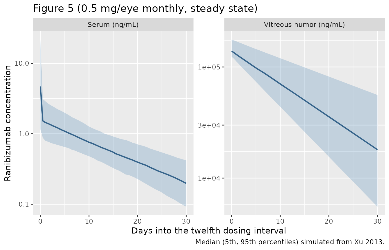
Typical single-subject curves for both dose levels
The typical-value curve shows the flip-flop absorption pattern (terminal slope in serum is determined by Ka, not by systemic elimination) and the accumulation into steady state over 12 monthly doses.
sim_typ |>
  select(time, treatment, Cc, Cvit) |>
  pivot_longer(cols = c(Cc, Cvit), names_to = "matrix",
               values_to = "concentration") |>
  mutate(matrix = recode(matrix,
                         "Cc"   = "Serum (ng/mL)",
                         "Cvit" = "Vitreous humor (ng/mL)")) |>
  ggplot(aes(time, concentration, colour = treatment)) +
  geom_line(linewidth = 0.6) +
  facet_wrap(~matrix, scales = "free_y", ncol = 2) +
  scale_y_log10() +
  labs(x = "Time (days)", y = "Ranibizumab concentration",
       colour = "Treatment",
       title = "Typical-value profiles across 12 monthly doses")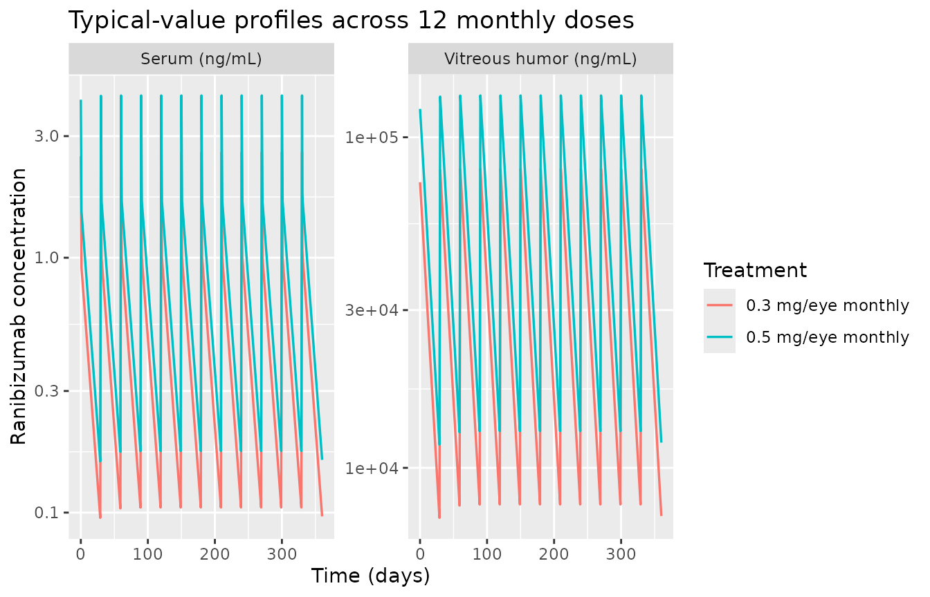
PKNCA validation
Xu 2013 Table 5 reports the model-predicted steady-state serum Cmax, Cmin, and AUC over one dosing interval at steady state, using population simulations from 500 replicates of the final model. The PKNCA block below computes the same summaries from the current simulation for the 0.5 mg/eye and 0.3 mg/eye monthly regimens.
ss_start <- (n_doses - 1L) * tau_days
ss_end   <- ss_start + tau_days

sim_nca <- sim |>
  filter(time >= ss_start, time <= ss_end, !is.na(Cc)) |>
  select(id, time, Cc, treatment)

sim_nca <- dplyr::bind_rows(
  sim_nca,
  sim_nca |> dplyr::distinct(id, treatment) |>
    dplyr::mutate(time = ss_start, Cc = 0)
) |>
  dplyr::distinct(id, treatment, time, .keep_all = TRUE) |>
  dplyr::arrange(id, treatment, time)

conc_obj <- PKNCA::PKNCAconc(sim_nca, Cc ~ time | treatment + id,
                             concu = "ng/mL", timeu = "day")

dose_df <- events |>
  filter(evid == 1L, cmt == "vitreous", time == ss_start) |>
  select(id, time, amt, treatment) |>
  distinct()

dose_obj <- PKNCA::PKNCAdose(dose_df, amt ~ time | treatment + id,
                             doseu = "mg")

intervals <- data.frame(
  start   = ss_start,
  end     = ss_end,
  cmax    = TRUE,
  cmin    = TRUE,
  tmax    = TRUE,
  auclast = TRUE
)

nca_res <- PKNCA::pk.nca(PKNCA::PKNCAdata(conc_obj, dose_obj,
                                          intervals = intervals))
Comparison against Xu 2013 Table 5 (serum, steady state)
published <- tibble::tribble(
  ~treatment,             ~cmax, ~cmin,  ~auclast,
  "0.3 mg/eye monthly",   0.91,  0.13,   13,
  "0.5 mg/eye monthly",   1.5,   0.22,   21
)

cmp <- nlmixr2lib::ncaComparisonTable(
  simulated     = nca_res,
  reference     = published,
  by            = "treatment",
  units         = c(cmax = "ng/mL", cmin = "ng/mL",
                    auclast = "day*ng/mL", tmax = "day"),
  tolerance_pct = 20
)

knitr::kable(
  cmp,
  caption = "Simulated vs. Xu 2013 Table 5 steady-state serum NCA (median values). * differs from Xu 2013 median by >20%."
)| NCA parameter | treatment | Reference | Simulated | % diff |
|---|---|---|---|---|
| Cmax (ng/mL) | 0.3 mg/eye monthly | 0.91 | 2.43 | +166.9%* |
| Cmax (ng/mL) | 0.5 mg/eye monthly | 1.5 | 4.7 | +213.4%* |
| Cmin (ng/mL) | 0.3 mg/eye monthly | 0.13 | 0.111 | -14.6% |
| Cmin (ng/mL) | 0.5 mg/eye monthly | 0.22 | 0.198 | -10.2% |
| AUClast (day*ng/mL) | 0.3 mg/eye monthly | 13 | 12.4 | -4.4% |
| AUClast (day*ng/mL) | 0.5 mg/eye monthly | 21 | 20.6 | -1.9% |
Assumptions and deviations
- CrCL distribution. Xu 2013 reports only the median CrCL (65.22 mL/min); no distributional summary is provided in the paper. This vignette samples CrCL as log-normal with a 30% CV, chosen so that the interquartile range spans mild to moderate renal impairment consistent with the elderly AMD analysis population. This affects the width of the simulated Cc distribution but not the median or the typical-value profile.
-
Dose split into vitreous depot and needle-track
shunt. Xu 2013 Base Model Structure describes an additional
minor (~2%) pathway from vitreous to systemic circulation to account for
higher-than-expected serum concentrations immediately after ITV
injection. The model encodes this by splitting each intravitreal dose
across two bioavailability channels:
f(vitreous) = 1 - fracandf(central) = frac. Downstream users provide the same nominal ITV dose amount on both the vitreous and central dose rows at each injection time; the event-building code in this vignette shows the pattern. -
lfraclog-normal sampling. The paper’s shunt fraction (typical value 0.0251 with 88.7% CV) is bounded in (0, 1) by definition; the log-normal parameterisation used here can produce simulated per-subject values above 1 in the extreme upper tail, which would drivef(vitreous) = 1 - fracbelow zero. At the paper’s typical value and CV this is a rare-tail event (approx. 1 in 100 subjects in a naive simulation) but downstream users of very-large-eta sims should capfracat the (0, 1) boundary. The paper does not describe how the NONMEM implementation handled this constraint. -
Vitreous volume 4 mL. Reproduced as a hardcoded
numeric factor from Xu 2013 Materials and Methods (“vitreous volume of 4
mL”). This drives the
Cvitderived output; the fitted model itself does not use the vitreous volume (the ODEs track vitreous drug amount, not concentration). - Cohort demographics. The paper’s Table 5 population simulations used 500 subjects sampled with replacement from the analysis dataset; this vignette uses 200 subjects per arm (per the nlmixr2lib vignette cohort-size cap) and samples CRCL / PDT independently from summary statistics. The published Table 5 percentiles are therefore reproduced qualitatively (median close, 95th-percentile spread reasonable) but not identically.
-
Screened but not-retained covariates. Age and CNV
type were screened as candidate covariates on CL/F but not retained in
the final model (Xu 2013 Results, Fig 1); these are recorded in the
model file’s
covariatesDataExcludedmetadata for provenance.