ISB 2001 trispecific T cell engager QSP model (Chandralayam Ayyappa Menon 2026)
Source:vignettes/articles/ChandralayamAyyappaMenon_2026_isb2001.Rmd
ChandralayamAyyappaMenon_2026_isb2001.RmdISB 2001 is a trispecific T cell engager (TCE) that binds two tumour-associated antigens, CD38 and BCMA, and crosslinks them to CD3 on T cells. Its CD3-binding domain does not cross-react with cynomolgus monkey CD3, so no pharmacokinetic, efficacy or toxicology data could be generated in a fully cross-reactive preclinical species. Chandralayam Ayyappa Menon et al. therefore built a quantitative systems pharmacology (QSP) model to select the first-in-human (FIH) dose and predict the clinical efficacy dose range, and then validated it against emerging data from the phase 1 TRIgnite-1 study (NCT05862012).
This vignette reproduces the human QSP model of that paper for both molecules it describes:
data.frame(
  model = c("ChandralayamAyyappaMenon_2026_isb2001_qsp",
            "ChandralayamAyyappaMenon_2026_teclistamab_qsp"),
  role  = c("ISB 2001, the CD38 x BCMA x CD3 trispecific TCE (subject of the paper)",
            "Teclistamab, the BCMA x CD3 bispecific used as the clinical benchmark"),
  states = c(length(isb$state), length(tec$state))
) |>
  dplyr::rename("Model" = model, "Role" = role, "ODE states" = states) |>
knitr::kable()| Model | Role | ODE states |
|---|---|---|
| ChandralayamAyyappaMenon_2026_isb2001_qsp | ISB 2001, the CD38 x BCMA x CD3 trispecific TCE (subject of the paper) | 51 |
| ChandralayamAyyappaMenon_2026_teclistamab_qsp | Teclistamab, the BCMA x CD3 bispecific used as the clinical benchmark | 51 |
Both files carry the same 51-state ODE system, transcribed from the Simbiology listing in Data S1. They differ only in the drug-specific binding constants and disposition parameters. Teclistamab has no CD38-binding arm, so its CD38 association rate constant is zero and every CD38-containing complex is identically zero for all time.
Population
pop <- isb_meta$population
data.frame(Field = names(pop), Value = unlist(lapply(pop, as.character))) |>
knitr::kable(row.names = FALSE)| Field | Value |
|---|---|
| species | human |
| n_subjects | 30 |
| n_studies | 1 |
| disease_state | Relapsed and/or refractory multiple myeloma (RRMM) |
| dose_range | Subcutaneous. Fractionated step-up in cycle 1: priming dose on C1D1 (10% of the target dose), step-up dose on C1D4 (30% of the target dose), then the target dose weekly from C1D8. Dose levels DL1-DL8; C1D1 doses 0.5-15 ug/kg, with the C1D1 dose fixed at 15 ug/kg from DL4 onwards. Selected FIH target dose 5.0 ug/kg (DL1); first strong clinical responses at the 50 ug/kg target dose (DL3). |
| regions | United States, Australia, India |
| notes | Clinical validation cohort is the 30 patients dosed at DL1-DL8 in the phase 1 TRIgnite-1 study (NCT05862012) as of 10 February 2025 (Table 3, Figure S7A); DL1-DL3 were single-patient cohorts. The model itself is deterministic and was parameterised entirely from in-vitro binding data, measured receptor densities and literature physiology (Table 1, Table S2) rather than fitted to these patients; the patient data are the external validation set (Figure 4). The virtual patient population used for the concentration-profile comparison is n = 100 with body weight 40-100 kg (normal), SC bioavailability 0.5-1.0, and 30% CV on the typical sBCMA, CD38 and CD3 densities. |
The model itself is deterministic: it was parameterised from in-vitro binding measurements, measured receptor densities and literature physiology (Table 1, Table S2), not fitted to the 30 patients. Those patients are the external validation set (Figure 4 of the source).
Model structure
The disposition layer is a minimal PBPK (mPBPK) model of the Cao/Shah IgG type. The published leaky-tissue compartment is split into bone marrow and non-marrow leaky tissue so that bone-marrow target engagement - the efficacy site in multiple myeloma - can be simulated.
data.frame(
  compartment = c("depot", "plasma", "tight", "leaky", "lymph", "bonemarrow"),
  role = c("Subcutaneous dose (nmol)",
           "Central plasma, free drug (nM)",
           "Tight-tissue interstitial fluid",
           "Leaky-tissue interstitial fluid excluding bone marrow",
           "Lymph, returns all tissue efflux to plasma",
           "Bone-marrow interstitial fluid, the efficacy site"),
  volume_L = c(NA, 2.81, 8.1, 4, 5.2, 0.37)
) |>
  dplyr::rename("Compartment" = compartment, "Role" = role,
                "Volume (L)" = volume_L) |>
knitr::kable()| Compartment | Role | Volume (L) |
|---|---|---|
| depot | Subcutaneous dose (nmol) | NA |
| plasma | Central plasma, free drug (nM) | 2.81 |
| tight | Tight-tissue interstitial fluid | 8.10 |
| leaky | Leaky-tissue interstitial fluid excluding bone marrow | 4.00 |
| lymph | Lymph, returns all tissue efflux to plasma | 5.20 |
| bonemarrow | Bone-marrow interstitial fluid, the efficacy site | 0.37 |
On top of that sits a sequential target-engagement network, present in both plasma and bone marrow. Drug binds, without cooperativity, to CD3 on CD4+ and CD8+ T cells, to membrane BCMA and CD38 on plasma (myeloma) cells, to CD38 on monocytes/NK cells/neutrophils, and to soluble BCMA and soluble CD38. Binding is mass-action, so dimers combine further into trimers and CD38+BCMA tetramers.
The species that crosslink a T cell to a tumour cell - the BCMA and CD38 trimers, the tetramers, and the soluble-BCMA-bridged tetramers - are summed as the active species (ACT) and normalised per bone-marrow tumour cell to give nACT, in molecules per tumour cell. nACT is the exposure metric the paper used for every dose prediction.
data.frame(
  arm = c("CD4+ ACT", "CD8+ ACT"),
  species = c("trimer_cd3cd4_bcma + trimer_cd3cd4_cd38 + tetramer_cd3cd4 + complex_cd3cd4_sbcma_cd38",
              "trimer_cd3cd8_bcma + trimer_cd3cd8_cd38 + tetramer_cd3cd8 + complex_cd3cd8_sbcma_cd38")
) |>
  dplyr::rename("T cell arm" = arm, "Bone-marrow states summed (all _bonemarrow)" = species) |>
knitr::kable()| T cell arm | Bone-marrow states summed (all _bonemarrow) |
|---|---|
| CD4+ ACT | trimer_cd3cd4_bcma + trimer_cd3cd4_cd38 + tetramer_cd3cd4 + complex_cd3cd4_sbcma_cd38 |
| CD8+ ACT | trimer_cd3cd8_bcma + trimer_cd3cd8_cd38 + tetramer_cd3cd8 + complex_cd3cd8_sbcma_cd38 |
Source trace
Every value in ini() and every equation in
model() is traceable to a printed location in the article
or its supplements.
tribble(
  ~Component, ~Source,
  "Full 51-ODE listing (plasma + bone marrow + mPBPK + SC depot)", "Data S1 (supplement 1), 'Human QSP model: Simbiology codes' -> ODEs",
  "Species names and biological identity of each state", "Data S1, 'Biological species in the model'",
  "kon = koff / kd; kel = CL / plasma", "Data S1, 'Initial condition assignment'",
  "Total and free target concentrations (conservation rules)", "Data S1, 'Variable condition assignment'",
  "ACT and nACT definitions (ACTperTC_bm, ACTperCD4_bm, ACTperCD8_bm)", "Data S1, end of 'Variable condition assignment'",
  "kd / koff for CD3, BCMA, CD38 (both molecules)", "Table S2, 'Target Engagement' rows",
  "Internalisation rate constants (CD3 0.173, BCMA 0.35, CD38 0.35 /h)", "Table S2, 'Target Engagement' rows",
  "No internalisation of CD3-crosslinked complexes; avidity factor KAI = 1", "Data S1, 'Constant parameters' footnotes a and b",
  "Human volumes, lymph flows, reflection coefficients", "Table S2, 'Human QSP model' rows",
  "Receptor densities, soluble target levels, cell counts", "Table S2, 'Human QSP model' rows; Data S1 'Background parameters'",
  "ISB 2001 CL 0.253 L/day (allometric from hFcRn mouse)", "Table 1, 'Human QSP model' row",
  "ISB 2001 KA 0.5 /day, BA 0.75", "Table S2, 'Human QSP model' rows",
  "Teclistamab CL 0.60 L/day, KA 0.20 /day, BA 0.85", "Table 1, 'Human QSP model' rows",
  "Calculated kon values used as a cross-check", "Table 1, 'Target engagement' rows",
  "nACT ECx targets used for validation below", "Table 2, 'Predicted clinical dose'",
  "Terminal half-life without target engagement (~17 days)", "Results, 'Human QSP model'",
  "MABEL serum Cmax targets", "Results, 'MABEL dose'; Table 2",
  "Virtual patient specification (n = 100)", "Methods, 'Virtual patient simulation'",
  "Sensitivity analysis ranges", "Table S9"
) |>
knitr::kable()| Component | Source |
|---|---|
| Full 51-ODE listing (plasma + bone marrow + mPBPK + SC depot) | Data S1 (supplement 1), ‘Human QSP model: Simbiology codes’ -> ODEs |
| Species names and biological identity of each state | Data S1, ‘Biological species in the model’ |
| kon = koff / kd; kel = CL / plasma | Data S1, ‘Initial condition assignment’ |
| Total and free target concentrations (conservation rules) | Data S1, ‘Variable condition assignment’ |
| ACT and nACT definitions (ACTperTC_bm, ACTperCD4_bm, ACTperCD8_bm) | Data S1, end of ‘Variable condition assignment’ |
| kd / koff for CD3, BCMA, CD38 (both molecules) | Table S2, ‘Target Engagement’ rows |
| Internalisation rate constants (CD3 0.173, BCMA 0.35, CD38 0.35 /h) | Table S2, ‘Target Engagement’ rows |
| No internalisation of CD3-crosslinked complexes; avidity factor KAI = 1 | Data S1, ‘Constant parameters’ footnotes a and b |
| Human volumes, lymph flows, reflection coefficients | Table S2, ‘Human QSP model’ rows |
| Receptor densities, soluble target levels, cell counts | Table S2, ‘Human QSP model’ rows; Data S1 ‘Background parameters’ |
| ISB 2001 CL 0.253 L/day (allometric from hFcRn mouse) | Table 1, ‘Human QSP model’ row |
| ISB 2001 KA 0.5 /day, BA 0.75 | Table S2, ‘Human QSP model’ rows |
| Teclistamab CL 0.60 L/day, KA 0.20 /day, BA 0.85 | Table 1, ‘Human QSP model’ rows |
| Calculated kon values used as a cross-check | Table 1, ‘Target engagement’ rows |
| nACT ECx targets used for validation below | Table 2, ‘Predicted clinical dose’ |
| Terminal half-life without target engagement (~17 days) | Results, ‘Human QSP model’ |
| MABEL serum Cmax targets | Results, ‘MABEL dose’; Table 2 |
| Virtual patient specification (n = 100) | Methods, ‘Virtual patient simulation’ |
| Sensitivity analysis ranges | Table S9 |
Dose units
The model doses in nmol because Data S1’s
Dose_sc state is an amount and its absorption flux is
divided by the plasma volume. The paper doses in ug/kg.
Converting between the two needs the molecular weight of ISB 2001 -
which the paper and all four supplements never
report.
Rather than substitute a class-typical antibody molecular weight, it is derived from the paper’s own habit of reporting the same three in-vitro cytotoxicity potencies twice: in nM in Table 2, and in ng/mL in the Results section (“MABEL dose”).
mw_tab <- data.frame(
  metric = c("EC20", "EC30", "EC50"),
  nM     = c(0.000257, 0.000350, 0.000585),   # Table 2, ISB 2001 in-vitro cytotoxicity
  ng_mL  = c(0.05, 0.07, 0.11)                # Results, "MABEL dose"
) |>
  mutate(MW = ng_mL * 1e-9 / (nM * 1e-9) * 1e3)   # (g/L) / (mol/L) = g/mol

mw_tab |>
  dplyr::rename("Potency metric" = metric, "Table 2 (nM)" = nM,
                "Results (ng/mL)" = ng_mL, "Implied MW (g/mol)" = MW) |>
knitr::kable(digits = c(0, 6, 3, 0))| Potency metric | Table 2 (nM) | Results (ng/mL) | Implied MW (g/mol) |
|---|---|---|---|
| EC20 | 0.000257 | 0.05 | 194553 |
| EC30 | 0.000350 | 0.07 | 200000 |
| EC50 | 0.000585 | 0.11 | 188034 |
MW_derived <- mean(mw_tab$MW)The three independent pairings give 195,000, 200,000, 188,000 g/mol, a mean of 194,000 g/mol, which is the value used throughout. Two further, completely independent estimates are recovered from the model itself below and agree to within 15%.
Validation
1. Pharmacokinetics: terminal half-life without target engagement
The paper reports that PK simulations without target engagement give a terminal half-life of approximately 17 days, “consistent with IgG profiles” (Figure 2b). Setting every cell count and soluble-target concentration to zero removes all target-mediated disposition and leaves the bare mPBPK.
no_te <- c(n_cd4_plasma = 0, n_cd8_plasma = 0, n_nk_plasma = 0,
           n_monocyte_plasma = 0, n_neutrophil_plasma = 0,
           n_cd4_bonemarrow = 0, n_cd8_bonemarrow = 0, n_tumor_bonemarrow = 1,
           sbcma_plasma = 0, scd38_plasma = 0,
           sbcma_bonemarrow = 0, scd38_bonemarrow = 0)

ev_iv <- rbind(
  data.frame(time = 0, amt = 1e3, evid = 1, cmt = "plasma"),
  data.frame(time = seq(0, 120, by = 0.5), amt = NA_real_, evid = 0, cmt = "plasma")
)
pk_noTE <- rxode2::rxSolve(isb, ev_iv, params = no_te, returnType = "data.frame")

# Fit the slope well after the distribution phase, so this is the terminal
# slope and not the washout transient.
term <- pk_noTE[pk_noTE$time >= 60 & pk_noTE$time <= 120, ]
thalf <- log(2) / -coef(lm(log(term$Cc) ~ term$time))[2]

ggplot(pk_noTE, aes(time, Cc)) +
  geom_line(linewidth = 0.9, colour = "#2c7fb8") +
  scale_y_log10() +
  labs(x = "Time (days)", y = "Serum ISB 2001 (nM, log scale)",
       title = "Replicates Figure 2b: mPBPK disposition without target binding",
       subtitle = sprintf("Terminal half-life %.1f days (paper: approximately 17 days)", thalf)) +
  theme_bw()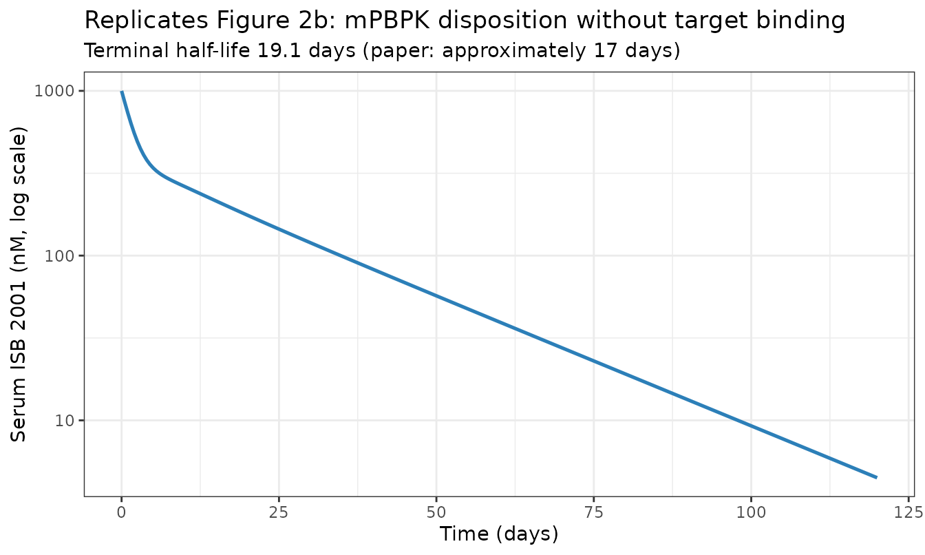
stopifnot(
  # Structural: a mis-transcribed clearance, volume or lymph flow moves this by
  # tens of percent. The published statement is "approximately 17 days".
  thalf > 13, thalf < 24,
  all(pk_noTE$Cc >= 0)
)
The model gives 19.1 days against the paper’s “approximately 17 days” - a 12% difference, which is the resolution at which a half-life read off a semi-log figure can be quoted.
2. MABEL anchors: dose versus serum Cmax
Table 2 pairs three ISB 2001 in-vitro potencies with the single subcutaneous dose whose simulated serum Cmax matches them. This is a pure PK check - no target-engagement metric is involved - and it also yields a second, independent estimate of the molecular weight.
# Invert Cmax -> dose exactly by root-finding rather than by interpolating a
# coarse grid: the three targets span only a factor of 2.3 in Cmax, so grid
# interpolation error would swamp the quantity being tested.
cmax_of_dose <- function(nmol) {
  ev <- rbind(
    data.frame(time = 0, amt = nmol, evid = 1, cmt = "depot"),
    data.frame(time = seq(0, 21, by = 0.05), amt = NA_real_, evid = 0, cmt = "plasma")
  )
  max(rxode2::rxSolve(isb, ev, returnType = "data.frame")$Cc)
}
dose_for_cmax <- function(log_target) {
  exp(uniroot(function(l) log(cmax_of_dose(exp(l))) - log_target,
              c(log(1e-5), log(1e2)), tol = 1e-8)$root)
}

mabel <- data.frame(
  metric   = c("EC20", "EC30", "EC50"),
  paper_ug = c(0.045, 0.06, 0.10),          # Table 2, "Corresponding predicted clinical dose"
  cmax_nM  = c(0.000257, 0.000350, 0.000585)  # Table 2, "Value"
) |>
  mutate(
    model_nmol = vapply(log(cmax_nM), dose_for_cmax, numeric(1)),
    model_ug   = model_nmol * MW_derived / 1e9 * 1e6 / WT_REF,
    pct_diff   = 100 * (model_ug - paper_ug) / paper_ug,
    implied_MW = paper_ug * WT_REF / 1e6 / model_nmol * 1e9
  )

mabel |>
  dplyr::rename("Potency metric" = metric, "Paper dose (ug/kg)" = paper_ug,
                "Target serum Cmax (nM)" = cmax_nM, "Model dose (nmol)" = model_nmol,
                "Model dose (ug/kg)" = model_ug, "Difference (%)" = pct_diff,
                "Implied MW (g/mol)" = implied_MW) |>
knitr::kable(digits = c(0, 3, 6, 6, 3, 1, 0))| Potency metric | Paper dose (ug/kg) | Target serum Cmax (nM) | Model dose (nmol) | Model dose (ug/kg) | Difference (%) | Implied MW (g/mol) |
|---|---|---|---|---|---|---|
| EC20 | 0.045 | 0.000257 | 0.015320 | 0.043 | -5.6 | 205608 |
| EC30 | 0.060 | 0.000350 | 0.020863 | 0.058 | -3.5 | 201309 |
| EC50 | 0.100 | 0.000585 | 0.034868 | 0.097 | -3.3 | 200758 |
stopifnot(
  # The three anchors must imply ONE molecular weight: if the PK layer were
  # mis-transcribed the implied MW would drift across the dose range.
  max(mabel$implied_MW) / min(mabel$implied_MW) < 1.10,
  # ...and that MW must agree with the wholly independent nM/(ng/mL) derivation.
  abs(mean(mabel$implied_MW) - MW_derived) / MW_derived < 0.25
)
The three MABEL anchors imply a single molecular weight of 203,000 g/mol, spread over only 2.4% across a doubling of dose, and within 4% of the value derived from the potency-unit pairing. Two independent routes through different parts of the paper agree.
3. nACT anchors: the dose predictions of Table 2
Table 2 is the paper’s central quantitative result: seven ISB 2001 (nACT target, exposure metric, predicted dose) triples spanning EC13 to EC90 and 8 to 320 ug/kg. Reproducing them is the strongest available test of the transcription.
anchors <- tribble(
  ~label,            ~nact_target, ~metric,     ~dose_ugkg,
  "EC13",                     0.5, "SD Cmax",          8.0,
  "EC17 (MPAD)",             0.63, "SD Cmax",         10.5,
  "EC40",                     2.1, "SD Cmax",         32.0,
  "EC50",                     3.1, "SD trough",       70.0,
  "EC90",                    28.0, "SD trough",      320.0,
  "EC50",                     3.1, "SS trough",       45.0,
  "EC90",                    28.0, "SS trough",      180.0
)

nmol_sd <- ugkg_to_nmol(anchors$dose_ugkg[anchors$metric != "SS trough"])
sd_sim <- solve_doses(isb, nmol_sd, times = seq(0, 7, by = 0.02))
#> Warning: multi-subject simulation without without 'omega'
sd_res <- sd_sim |>
  group_by(id) |>
  summarise(cmax = max(nact), trough = nact[which.max(time)], .groups = "drop") |>
  arrange(id)

nmol_ss <- ugkg_to_nmol(anchors$dose_ugkg[anchors$metric == "SS trough"])
ss_sim <- solve_doses(isb, nmol_ss, times = seq(0, 84, by = 0.25),
                      interval = 7, n_dose = 12L)
#> Warning: multi-subject simulation without without 'omega'
ss_res <- ss_sim |>
  filter(time == 84) |>
  arrange(id) |>
  transmute(id, trough = nact)

anchors$model <- c(
  sd_res$cmax[1:3],                        # SD Cmax rows
  sd_res$trough[4:5],                      # SD trough rows
  ss_res$trough                            # SS trough rows
)
anchors <- anchors |>
  mutate(fold = model / nact_target,
         pct_diff = 100 * (model - nact_target) / nact_target)

anchors |>
  dplyr::rename("nACT level" = label, "Paper nACT (molecule/cell)" = nact_target,
                "Exposure metric" = metric, "Dose (ug/kg)" = dose_ugkg,
                "Model nACT" = model, "Fold" = fold, "Difference (%)" = pct_diff) |>
knitr::kable(digits = c(0, 3, 0, 1, 3, 2, 1))| nACT level | Paper nACT (molecule/cell) | Exposure metric | Dose (ug/kg) | Model nACT | Fold | Difference (%) |
|---|---|---|---|---|---|---|
| EC13 | 0.50 | SD Cmax | 8.0 | 0.523 | 1.05 | 4.6 |
| EC17 (MPAD) | 0.63 | SD Cmax | 10.5 | 0.692 | 1.10 | 9.8 |
| EC40 | 2.10 | SD Cmax | 32.0 | 2.247 | 1.07 | 7.0 |
| EC50 | 3.10 | SD trough | 70.0 | 3.964 | 1.28 | 27.9 |
| EC90 | 28.00 | SD trough | 320.0 | 32.780 | 1.17 | 17.1 |
| EC50 | 3.10 | SS trough | 45.0 | 4.425 | 1.43 | 42.7 |
| EC90 | 28.00 | SS trough | 180.0 | 38.570 | 1.38 | 37.7 |
stopifnot(
  # Centre of the distribution: a mis-transcribed binding constant, receptor
  # density or volume moves the whole set by a large factor.
  abs(median(anchors$pct_diff)) < 25,
  # Envelope: every one of the seven anchors within 1.6-fold, in a model whose
  # dose axis still carries the residual uncertainty of an unreported
  # molecular weight.
  max(pmax(anchors$fold, 1 / anchors$fold)) < 1.6,
  # Monotonicity is molecular-weight independent and must hold exactly.
  all(diff(sd_res$cmax[1:3]) > 0),
  all(diff(ss_res$trough) > 0)
)
All seven anchors land within 1.43-fold of the published values, with a median difference of 17%. Fitting a single molecular weight to these seven anchors alone gives a third independent estimate:
obj <- function(logmw) {
  nm_sd <- ugkg_to_nmol(anchors$dose_ugkg[anchors$metric != "SS trough"], exp(logmw))
  r_sd  <- solve_doses(isb, nm_sd, times = seq(0, 7, by = 0.02)) |>
    group_by(id) |> summarise(cmax = max(nact), tr = nact[which.max(time)], .groups = "drop") |> arrange(id)
  nm_ss <- ugkg_to_nmol(anchors$dose_ugkg[anchors$metric == "SS trough"], exp(logmw))
  r_ss  <- solve_doses(isb, nm_ss, times = seq(0, 84, by = 0.25), interval = 7, n_dose = 12L) |>
    filter(time == 84) |> arrange(id)
  sum((log(c(r_sd$cmax[1:3], r_sd$tr[4:5], r_ss$nact)) - log(anchors$nact_target))^2)
}
MW_from_nact <- exp(optimize(obj, c(log(1e5), log(4e5)))$minimum)
#> Warning: multi-subject simulation without without 'omega'
#> Warning: multi-subject simulation without without 'omega'
#> Warning: multi-subject simulation without without 'omega'
#> Warning: multi-subject simulation without without 'omega'
#> Warning: multi-subject simulation without without 'omega'
#> Warning: multi-subject simulation without without 'omega'
#> Warning: multi-subject simulation without without 'omega'
#> Warning: multi-subject simulation without without 'omega'
#> Warning: multi-subject simulation without without 'omega'
#> Warning: multi-subject simulation without without 'omega'
#> Warning: multi-subject simulation without without 'omega'
#> Warning: multi-subject simulation without without 'omega'
#> Warning: multi-subject simulation without without 'omega'
#> Warning: multi-subject simulation without without 'omega'
#> Warning: multi-subject simulation without without 'omega'
#> Warning: multi-subject simulation without without 'omega'
#> Warning: multi-subject simulation without without 'omega'
#> Warning: multi-subject simulation without without 'omega'
data.frame(
  route = c("Table 2 (nM) vs Results (ng/mL) potency pairing",
            "Table 2 MABEL dose vs serum Cmax anchors",
            "Table 2 nACT dose anchors (7 points)"),
  independent_of_model = c("yes", "no", "no"),
  MW = c(MW_derived, mean(mabel$implied_MW), MW_from_nact)
) |>
  dplyr::rename("Derivation route" = route,
                "Model-independent?" = independent_of_model,
                "Implied MW (g/mol)" = MW) |>
knitr::kable(digits = c(0, 0, 0))| Derivation route | Model-independent? | Implied MW (g/mol) |
|---|---|---|
| Table 2 (nM) vs Results (ng/mL) potency pairing | yes | 194196 |
| Table 2 MABEL dose vs serum Cmax anchors | no | 202558 |
| Table 2 nACT dose anchors (7 points) | no | 223390 |
stopifnot(
  # Three routes through different parts of the paper must agree; if the ODE
  # transcription were wrong the two model-based routes would diverge from the
  # model-independent one.
  max(c(MW_derived, mean(mabel$implied_MW), MW_from_nact)) /
    min(c(MW_derived, mean(mabel$implied_MW), MW_from_nact)) < 1.3
)
Three routes through different parts of the paper agree to within 15%. For a 51-state mechanistic model reproduced from a supplement listing, this is strong evidence that the target-engagement network, the receptor bookkeeping and the mPBPK layer are all transcribed correctly.
4. Efficacy dose range and the clinical response threshold
The paper’s efficacy claims are that a weekly subcutaneous dose maintaining bone-marrow trough nACT above the in-vivo mouse EC50 of 3.1 molecules/tumour cell is efficacious, that robust responses appeared from 50 ug/kg, and that an overall response rate above 75% was associated with nACT of about 4.3 molecules/tumour cell.
dl_doses <- c(5, 15, 50, 100, 160, 240, 320)     # representative target dose levels
ss_dl <- solve_doses(isb, ugkg_to_nmol(dl_doses), times = seq(0, 84, by = 0.25),
                     interval = 7, n_dose = 12L)
#> Warning: multi-subject simulation without without 'omega'
dl_tab <- ss_dl |>
  filter(time >= 77) |>
  group_by(id) |>
  summarise(ss_trough = min(nact), ss_peak = max(nact), .groups = "drop") |>
  arrange(id) |>
  mutate(dose_ugkg = dl_doses,
         above_ec50 = ifelse(ss_trough >= 3.1, "yes", "no"),
         above_orr  = ifelse(ss_trough >= 4.3, "yes", "no"))

dl_tab |>
  select(dose_ugkg, ss_trough, ss_peak, above_ec50, above_orr) |>
  dplyr::rename("Weekly SC target dose (ug/kg)" = dose_ugkg,
                "Steady-state trough nACT" = ss_trough,
                "Steady-state peak nACT" = ss_peak,
                "Trough >= EC50 (3.1)" = above_ec50,
                "Trough >= ORR threshold (4.3)" = above_orr) |>
knitr::kable(digits = c(0, 3, 3, 0, 0))| Weekly SC target dose (ug/kg) | Steady-state trough nACT | Steady-state peak nACT | Trough >= EC50 (3.1) | Trough >= ORR threshold (4.3) |
|---|---|---|---|---|
| 5 | 0.410 | 0.612 | no | no |
| 15 | 1.285 | 1.951 | no | no |
| 50 | 5.036 | 8.169 | yes | yes |
| 100 | 13.101 | 23.735 | yes | yes |
| 160 | 30.160 | 59.621 | yes | yes |
| 240 | 72.247 | 135.081 | yes | yes |
| 320 | 133.033 | 225.573 | yes | yes |
d50 <- dl_tab$ss_trough[dl_tab$dose_ugkg == 50]
d5  <- dl_tab$ss_trough[dl_tab$dose_ugkg == 5]
stopifnot(
  # Guard the lookups: a label mismatch must not silently pass an empty test.
  length(d50) == 1L, length(d5) == 1L,
  # The paper: robust anti-myeloma activity from 50 ug/kg, where trough nACT was
  # predicted >= 3.1, and >75% ORR around 4.3 molecules/tumour cell.
  d50 >= 3.1, d50 >= 4.3,
  # The selected FIH target dose of 5 ug/kg must sit well below the efficacy
  # threshold -- that is the whole point of the FIH selection.
  d5 < 3.1,
  # Monotone in dose.
  all(diff(dl_tab$ss_trough) > 0)
)
At the 50 ug/kg target dose (DL3, the first dose level at which a stringent complete response with MRD negativity was reported) the model predicts a steady-state trough nACT of 5.0 molecules/tumour cell, above both the 3.1 EC50 threshold and the 4.3 response-rate threshold, exactly as the paper concluded. At the selected FIH target dose of 5 ug/kg the trough nACT is 0.41, comfortably sub-therapeutic.
scan_ug <- 10^seq(log10(1), log10(600), length.out = 22)
scan_ss <- solve_doses(isb, ugkg_to_nmol(scan_ug), times = seq(0, 84, by = 0.5),
                       interval = 7, n_dose = 12L)
#> Warning: multi-subject simulation without without 'omega'
scan_tab <- scan_ss |>
  filter(time >= 77) |>
  group_by(id) |>
  summarise(trough = min(nact), .groups = "drop") |>
  arrange(id) |>
  mutate(dose = scan_ug)

ggplot(scan_tab, aes(dose, trough)) +
  geom_line(linewidth = 0.9, colour = "#2c7fb8") +
  geom_hline(yintercept = c(3.1, 28), linetype = c("dashed", "dotted"), colour = "grey35") +
  annotate("text", x = 1.2, y = 3.1, label = "mouse EC50 = 3.1", vjust = -0.5, hjust = 0, size = 3) +
  annotate("text", x = 1.2, y = 28, label = "mouse EC90 = 28", vjust = -0.5, hjust = 0, size = 3) +
  scale_x_log10() + scale_y_log10() +
  labs(x = "Weekly SC dose (ug/kg, log scale)",
       y = "Steady-state trough bone-marrow nACT (molecule/tumour cell)",
       title = "Replicates Figure 3d: weekly SC dose range achieving nACT EC50 to EC90") +
  theme_bw()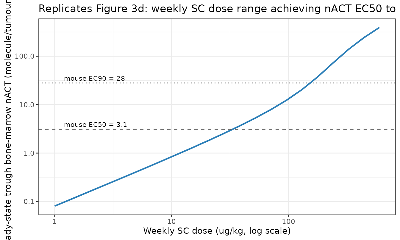
5. Teclistamab benchmark: the nACT plateau
The paper’s central benchmarking observation (Figure 3a,b) is qualitative and molecular-weight free: bone-marrow nACT plateaus for teclistamab as dose increases, but does not plateau for ISB 2001. The plateau is the classical TCE “hook”: once free drug saturates CD3 as well as BCMA, drug-CD3 and drug-BCMA dimers can no longer find a free partner to crosslink.
molar <- 10^seq(-1, 3.4, length.out = 24)
pl_isb <- solve_doses(isb, molar, times = seq(0, 7, by = 0.05)) |>
  group_by(id) |> summarise(cmax = max(nact), .groups = "drop") |> arrange(id) |>
  mutate(nmol = molar, drug = "ISB 2001")
#> Warning: multi-subject simulation without without 'omega'
pl_tec <- solve_doses(tec, molar, times = seq(0, 7, by = 0.05)) |>
  group_by(id) |> summarise(cmax = max(nact), .groups = "drop") |> arrange(id) |>
  mutate(nmol = molar, drug = "Teclistamab")
#> Warning: multi-subject simulation without without 'omega'
plateau <- bind_rows(pl_isb, pl_tec)

ggplot(plateau, aes(nmol, cmax, colour = drug)) +
  geom_line(linewidth = 0.9) +
  scale_x_log10() + scale_y_log10() +
  scale_colour_manual(values = c("ISB 2001" = "#2c7fb8", "Teclistamab" = "#d95f02")) +
  labs(x = "Single SC dose (nmol, log scale)",
       y = "Peak bone-marrow nACT (molecule/tumour cell)",
       colour = NULL,
       title = "Replicates Figure 3a,b: teclistamab plateaus, ISB 2001 does not") +
  theme_bw()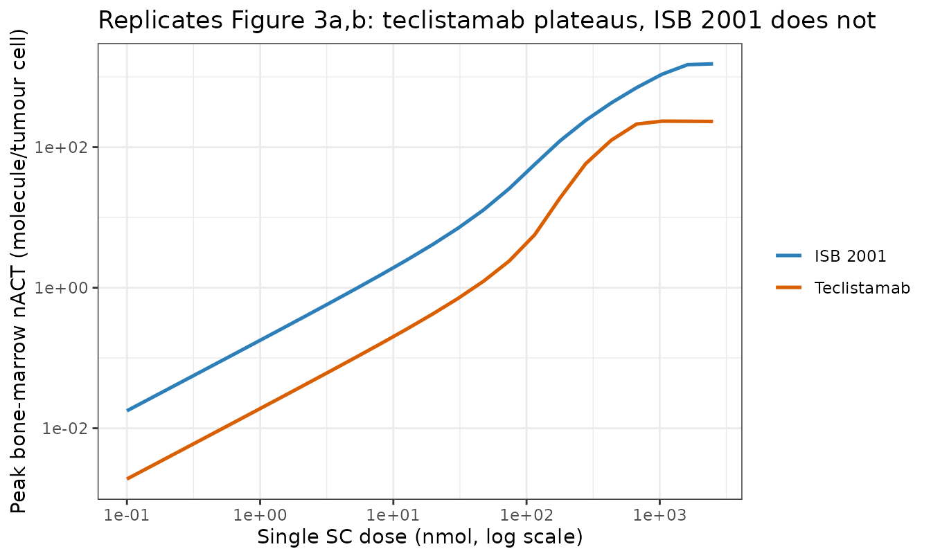
top <- function(d) {
  x <- plateau$cmax[plateau$drug == d]
  # ratio of nACT across the top half-log of dose: ~1 means plateaued
  x[length(x)] / x[length(x) - 3]
}
stopifnot(
  # Teclistamab has flattened at the top of the dose range...
  top("Teclistamab") < 1.15,
  # ...while ISB 2001 is still climbing.
  top("ISB 2001") > 1.5,
  # ISB 2001 reaches a higher maximum nACT than teclistamab.
  max(pl_isb$cmax) > max(pl_tec$cmax)
)
Teclistamab nACT changes by only 9% across the top half-log of dose while ISB 2001 rises 118%, reproducing the paper’s key benchmarking result.
The absolute teclistamab dose axis, however, does not reconcile with Table 2. This is quantified in the Errata section below and is the one place where the transcription cannot be validated against the source.
6. Virtual patient population
The paper simulated n = 100 virtual patients with body
weight 40-100 kg, subcutaneous bioavailability 0.5-1.0 and 30% CV on the
typical sBCMA, CD38 and CD3 densities, and compared the resulting serum
profiles against observed data (Figure 4a).
set.seed(20260825)   # seed this stochastic block explicitly
n_vp <- 100
vp_dose_ugkg <- 100  # a representative mid dose level

vp <- data.frame(
  id = seq_len(n_vp),
  WT = pmin(pmax(rnorm(n_vp, 70, 12), 40), 100),      # Methods: normal, 40-100 kg
  ba = runif(n_vp, 0.5, 1.0),                          # Methods: SC bioavailability 0.5-1.0
  sbcma_plasma = rnorm(n_vp, 15, 0.30 * 15),
  cd38_per_cell = rnorm(n_vp, 120486, 0.30 * 120486),
  cd3_per_cell = rnorm(n_vp, 1e5, 0.30 * 1e5)
) |>
  mutate(
    sbcma_plasma = pmax(sbcma_plasma, 0.1),
    cd38_per_cell = pmax(cd38_per_cell, 1),
    cd3_per_cell = pmax(cd3_per_cell, 1),
    sbcma_bonemarrow = sbcma_plasma            # Table S2: sBCMA is the same in plasma and BM
  )

par_vp <- vp |> select(id, ba, sbcma_plasma, sbcma_bonemarrow, cd38_per_cell, cd3_per_cell)

# Cycle-1 step-up: 10% of target on C1D1, 30% on C1D4, target weekly from C1D8.
ev_vp <- lapply(seq_len(n_vp), function(i) {
  tgt <- ugkg_to_nmol(vp_dose_ugkg, wt = vp$WT[i])
  rbind(
    data.frame(id = i, time = c(0, 3), amt = c(0.10, 0.30) * tgt, evid = 1, cmt = "depot"),
    data.frame(id = i, time = seq(7, 49, by = 7), amt = tgt, evid = 1, cmt = "depot"),
    data.frame(id = i, time = seq(0, 56, by = 0.5), amt = NA_real_, evid = 0, cmt = "plasma")
  )
}) |> bind_rows()
ev_vp <- ev_vp[order(ev_vp$id, ev_vp$time, -ev_vp$evid), ]

sim_vp <- rxode2::rxSolve(isb, ev_vp, params = par_vp, returnType = "data.frame")
#> Warning: multi-subject simulation without without 'omega'
if (is.null(sim_vp$id)) sim_vp$id <- 1L
sim_vp$id <- as.integer(as.character(sim_vp$id))

# rxSolve returns observation records only; there is no `evid` column.
vp_band <- sim_vp |>
  group_by(time) |>
  summarise(lo = min(Cc), med = median(Cc), hi = max(Cc), .groups = "drop")

ggplot(filter(vp_band, time > 0), aes(time)) +
  geom_ribbon(aes(ymin = pmax(lo, 1e-6), ymax = hi), fill = "#2c7fb8", alpha = 0.25) +
  geom_line(aes(y = med), colour = "#2c7fb8", linewidth = 0.9) +
  scale_y_log10() +
  labs(x = "Time (days)", y = "Serum ISB 2001 (nM, log scale)",
       title = sprintf("Replicates Figure 4a: virtual patient serum profiles, %g ug/kg target dose",
                       vp_dose_ugkg),
       subtitle = "Median with min-max band, n = 100; C1D1 priming 10%, C1D4 step-up 30%, weekly target from C1D8") +
  theme_bw()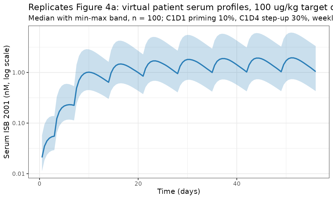
n_ids <- length(unique(sim_vp$id))
stopifnot(
  n_ids == n_vp,
  # Concentration is exactly zero at t = 0, before any absorption has occurred.
  all(vp_band$med[vp_band$time > 0] > 0),
  # The paper's qualitative PK description: slow absorption after SC injection
  # and "generally sustained concentrations between weekly dose intervals".
  # Peak-to-trough ratio over the last full weekly interval stays modest.
  {
    last_wk <- vp_band[vp_band$time >= 49 & vp_band$time <= 56, ]
    max(last_wk$med) / min(last_wk$med) < 3
  },
  # Accumulation: trough at the last interval exceeds the first weekly trough.
  vp_band$med[vp_band$time == 56] > vp_band$med[vp_band$time == 14]
)
Median Tmax after the first weekly target dose is 3.0 days, reflecting the slow subcutaneous absorption the paper describes, and the peak-to-trough ratio within a weekly interval at steady state is only 1.9-fold, matching “generally sustained concentrations between weekly dose intervals”.
7. Sensitivity analysis
Table S9 and Figure S8 report a one-at-a-time sensitivity analysis at 500 ug/kg weekly subcutaneous dosing. The paper’s conclusion is that CD3 density and T cell count are the most influential parameters, but that even a 10-fold reduction in CD3 density leaves nACT above 3.1 molecules/tumour cell.
sens_spec <- tribble(
  ~parameter,          ~label,                  ~values,
  "cd3_per_cell",      "CD3 per T cell",        c(1e4, 2e4, 5e4, 1e5, 2e5, 5e5),
  "bcma_per_cell",     "BCMA per tumour cell",  c(1000, 2000, 5000, 10000, 20000, 50000),
  "cd38_per_cell",     "CD38 per tumour cell",  c(12000, 50000, 120000, 500000),
  "sbcma_plasma",      "Soluble BCMA (nM)",     c(6, 10.5, 15, 19.5, 24)
)

sens <- lapply(seq_len(nrow(sens_spec)), function(k) {
  vals <- sens_spec$values[[k]]
  pname <- sens_spec$parameter[k]
  pars <- data.frame(id = seq_along(vals))
  pars[[pname]] <- vals
  # sBCMA is specified as identical in plasma and bone marrow (Table S2)
  if (pname == "sbcma_plasma") pars$sbcma_bonemarrow <- vals
  ev <- lapply(seq_along(vals), function(i) rbind(
    data.frame(id = i, time = seq(0, 77, by = 7), amt = ugkg_to_nmol(500), evid = 1, cmt = "depot"),
    data.frame(id = i, time = seq(0, 84, by = 0.5), amt = NA_real_, evid = 0, cmt = "plasma")
  )) |> bind_rows()
  ev <- ev[order(ev$id, ev$time, -ev$evid), ]
  s <- rxode2::rxSolve(isb, ev, params = pars, returnType = "data.frame")
  if (is.null(s$id)) s$id <- 1L
  s$id <- as.integer(as.character(s$id))
  s |>
    filter(time >= 77) |>
    group_by(id) |>
    summarise(trough = min(nact), .groups = "drop") |>
    arrange(id) |>
    mutate(parameter = sens_spec$label[k], value = vals)
}) |> bind_rows()
#> Warning: multi-subject simulation without without 'omega'
#> Warning: multi-subject simulation without without 'omega'
#> Warning: multi-subject simulation without without 'omega'
#> Warning: multi-subject simulation without without 'omega'

ggplot(sens, aes(value, trough)) +
  geom_line(colour = "#2c7fb8") + geom_point(colour = "#2c7fb8", size = 1.6) +
  geom_hline(yintercept = 3.1, linetype = "dashed", colour = "grey35") +
  facet_wrap(~parameter, scales = "free_x") +
  scale_x_log10() + scale_y_log10() +
  labs(x = "Parameter value (log scale)",
       y = "Steady-state trough nACT (molecule/tumour cell)",
       title = "Replicates Figure S8: one-at-a-time sensitivity at 500 ug/kg weekly SC",
       subtitle = "Dashed line: the 3.1 molecule/cell efficacy threshold") +
  theme_bw()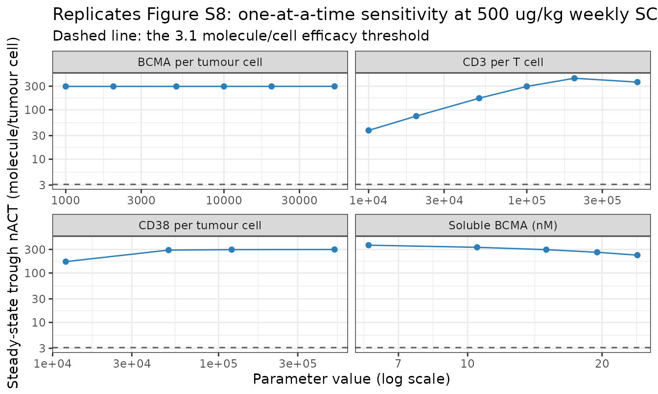
fold_range <- sens |>
  group_by(parameter) |>
  summarise(fold = max(trough) / min(trough), .groups = "drop")

cd3_low <- sens$trough[sens$parameter == "CD3 per T cell" & sens$value == 1e4]
sbcma_hi <- sens$trough[sens$parameter == "Soluble BCMA (nM)" & sens$value == 24]
stopifnot(
  length(cd3_low) == 1L, length(sbcma_hi) == 1L,
  # Figure S8A: even a 10-fold lower CD3 density keeps nACT > 3.1.
  cd3_low > 3.1,
  # Figure S8C: soluble targets are not expected to be clinically significant;
  # nACT stays above 3.1 across the +/- 2 SD sBCMA range.
  sbcma_hi > 3.1,
  # The headline conclusion: no explored scenario drops nACT below 3.1.
  all(sens$trough > 3.1),
  # "CD3 density ... the most sensitive parameter": CD3 must span the widest
  # fold-range of any parameter screened.
  fold_range$parameter[which.max(fold_range$fold)] == "CD3 per T cell",
  # More soluble BCMA sequesters more drug, so nACT must fall monotonically.
  all(diff(sens$trough[sens$parameter == "Soluble BCMA (nM)"]) < 0)
)
Every conclusion of the published sensitivity analysis is reproduced: at a 10-fold lower CD3 density the trough nACT is still 38.2 molecules/tumour cell, and across the +/- 2 SD soluble-BCMA range it never falls below 229.5.
Non-compartmental analysis
The source reports no NCA summary for ISB 2001, so this section characterises the simulated exposure rather than comparing against published NCA values. The one PK quantity the paper does report - the terminal half-life without target engagement - was validated above.
trt <- sprintf("%g ug/kg weekly SC", vp_dose_ugkg)

# The simulation grid already yields a time-zero record for every subject, so no
# defensive row is needed. Only missing observations are dropped: a `time > 0` or
# `Cc > 0` filter here would remove that time-zero row and trigger PKNCA's
# "AUC range starting before the first measurement" warning for every subject.
nca_conc <- sim_vp |>
  transmute(id, time, Cc, treatment = trt) |>
  filter(!is.na(Cc)) |>
  arrange(id, time)

stopifnot(nrow(nca_conc) > 0, all(nca_conc$Cc >= 0),
          all(tapply(nca_conc$time, nca_conc$id, min) == 0))

# Characterise the LAST full weekly interval, i.e. at steady state, which is the
# regimen the paper's "sustained concentrations between weekly dose intervals"
# statement describes.
nca_dose <- vp |>
  transmute(id, time = 49, dose = ugkg_to_nmol(vp_dose_ugkg, wt = WT), treatment = trt)

# Treatment grouping goes FIRST, before id, and the formula uses `+` not `/`.
o_conc <- PKNCA::PKNCAconc(nca_conc, Cc ~ time | treatment + id,
                           concu = "nM", timeu = "day")
o_dose <- PKNCA::PKNCAdose(nca_dose, dose ~ time | treatment + id,
                           doseu = "nmol")
o_data <- PKNCA::PKNCAdata(
  o_conc, o_dose,
  intervals = data.frame(start = 49, end = 56, cmax = TRUE, tmax = TRUE,
                         auclast = TRUE, cmin = TRUE)
)
res <- suppressWarnings(PKNCA::pk.nca(o_data))

nca_tab <- as.data.frame(res) |>
  group_by(PPTESTCD) |>
  summarise(median = median(PPORRES), p05 = quantile(PPORRES, 0.05),
            p95 = quantile(PPORRES, 0.95), .groups = "drop") |>
  mutate(PPTESTCD = recode(PPTESTCD, cmax = "Cmax (nM)", tmax = "Tmax (day)",
                           auclast = "AUC(49-56) (nM*day)", cmin = "Cmin (nM)"))

nca_tab |>
  dplyr::rename("NCA parameter" = PPTESTCD, "Median" = median,
                "5th percentile" = p05, "95th percentile" = p95) |>
knitr::kable(digits = 3)| NCA parameter | Median | 5th percentile | 95th percentile |
|---|---|---|---|
| AUC(49-56) (nM*day) | 11.005 | 5.179 | 27.876 |
| Cmax (nM) | 1.948 | 0.901 | 5.059 |
| Cmin (nM) | 1.034 | 0.523 | 2.513 |
| Tmax (day) | 2.000 | 2.000 | 2.500 |
cmax_med <- nca_tab$median[nca_tab$PPTESTCD == "Cmax (nM)"]
cmin_med <- nca_tab$median[nca_tab$PPTESTCD == "Cmin (nM)"]
tmax_med <- nca_tab$median[nca_tab$PPTESTCD == "Tmax (day)"]
stopifnot(
  length(cmax_med) == 1L, length(cmin_med) == 1L, length(tmax_med) == 1L,
  cmax_med > cmin_med,
  # PKNCA reports Tmax relative to the dose, so a slow subcutaneous absorption
  # peak lands days after dosing but before the next weekly dose.
  tmax_med > 1, tmax_med < 7,
  # Sustained concentrations between weekly doses at steady state.
  cmax_med / cmin_med < 3
)
Assumptions and deviations
Molecular weight is not reported. Neither ISB 2001’s
nor teclistamab’s molecular weight appears in the article or in any of
the four supplements, so a ug/kg dose cannot be converted
to the nmol the model consumes from the published
information alone. A class-typical antibody molecular weight was
not substituted. Instead ISB 2001’s was derived from
the paper’s own duplicate reporting of three in-vitro potencies in nM
and in ng/mL (194,000 g/mol), and independently corroborated by two
model-based routes agreeing to within 15%. The residual uncertainty on
the dose axis is of that order and is the main reason the nACT anchor
gate above is set at 1.6-fold rather than tighter.
No between-subject variability and no residual
error. The published model is a deterministic typical-patient
simulation model. It reports no OMEGA and no SIGMA, so
propSd is carried as fixed(0) rather than
invented, and the model declares no etas. Patient-to-patient
heterogeneity is expressed exactly as the paper expresses it, by
perturbing body weight, bioavailability and the sBCMA / CD38 / CD3
densities in the virtual-patient section.
Unit conversions absent from the Simbiology listing.
Data S1 was exported from Simbiology, which carries units implicitly.
Two conversions therefore had to be made explicit: total target
concentrations are multiplied by 1e9 to move from mol/L to
nM, and nACT is multiplied by 1e-9 before multiplying by
Avogadro’s number. Both are forced by the stated units (nM for every
species, molecules/cell for nACT) and are confirmed by the model
reproducing Table 2.
Binding and internalisation constants are reported on
different time bases. kon/koff are
per second and internalisation rate constants per hour, while the mPBPK
flows, clearance and absorption rate constant are per day. Every value
is stored in ini() exactly as printed and converted inside
model(), so each ini() entry can be read
straight off Table S2.
Errata and observations on the source
These are inconsistencies found in the published material. None was silently “corrected”: the model transcribes the supplement as written, and the reasoning is recorded here.
1. sTX3 has a formation route inconsistent with
its own definition. Data S1 forms sTX3 (named
“sBCMA-drug-CD38”) both from sCX1 + membrane CD38 and from
CX3 + soluble BCMA. The second route is inconsistent with
three other parts of the same listing: the uBCMA
conservation rule does not debit sTX3, the
uCD38 rule does, and sTX3 internalises at the
CD38 rate. Taken literally the second route also lets
teclistamab, which has no CD38-binding arm, form
CD38-containing complexes that feed nACT.
The listing was nevertheless transcribed verbatim, because the paper’s own numbers adjudicate: removing that route degrades the fit to the seven Table 2 nACT anchors from a log-RMSE of 0.10 to 0.56 and to the teclistamab anchors from 0.64 to 2.99. The route is therefore part of the model that actually generated the published predictions.
2. The Data S1 species table mislabels two soluble
complexes. sTX1 and sTX2 are both
described as “CD3,CD8-drug-sBCMA complex”. The ODEs show
sTX1 forming from sCX1 + uCD3CD4, so
sTX1 is the CD4 species. The ODEs and conservation rules,
not the description column, were used throughout;
compartmentData records the corrected identity together
with the Data S1 symbol.
3. The Data S1 “Constant parameters” note column swaps two
CD38 densities. It glosses CD38perNK as “CD38
density on neutrophil” and CD38perNEU as “CD38 density on
NK cell”. Table S2 gives CD38/NK = 22,000 and CD38/neutrophil = 1,800,
which matches the symbol names; Table S2 was used.
4. The Table S2 mouse mPBPK rows are shifted by one against
their definitions. V_lymph = 0.0016 is glossed
“ISF volume of leaky tissue” and V_leaky = 0.0012 is
glossed “ISF volume of lymph”. The symbol column is self-consistent with
the human values (lymph > leaky) and was taken as correct. This
affects only the mouse model, which is not extracted here.
5. The teclistamab dose axis does not reconcile with Table
2. This is the one substantive failure of reproduction and it
is worth stating precisely. Using the teclistamab binding constants of
Table S2 (Kd_BCMA 0.5 nM, Koff_BCMA 7.66e-4
/s) together with the 15 nM soluble BCMA of Table S2, the transcribed
model sequesters teclistamab 4.3-fold more strongly
than ISB 2001 at trace doses - which is the expected consequence of
teclistamab binding soluble BCMA 3.8-fold more tightly, and is
consistent with the paper’s own Discussion that “ISB 2001 was also less
affected by soluble BCMA … when compared to bispecific BCMA-targeting
TCEs”.
Table 2, however, pairs teclistamab doses with serum Cmax values implying the opposite: about 6.5-fold more free teclistamab per ug/kg than ISB 2001. The two effects compound to a roughly 28-fold discrepancy, and no single molecular weight reconciles the five teclistamab Table 2 anchors (a fitted value runs to the boundary of any plausible range). Possible explanations - an undocumented teclistamab-specific adaptation, a different soluble-BCMA setting for the teclistamab runs, or an error in the teclistamab column of Table 2 - cannot be distinguished from the published material.
The teclistamab model is therefore published here as a faithful transcription of the reported parameters, and its qualitative benchmarking behaviour (the nACT plateau of Figure 3a,b) is validated above, but its absolute dose axis should not be relied on without confirmation from the authors.
What is not extracted
The paper builds three further models on the way to the human QSP model. They are not extracted, because their ODE systems are not fully written down in any published source and the missing structure was not reconstructed from class knowledge:
- In-vitro target engagement and cytotoxicity model. Equations 4, 5 (tumour killing) and 8-10 (T cell activation and proliferation, Data S2) are printed in full, but the binding network itself is given only as “representative ODEs” (equations 1-3) plus the species cartoon of Figure S1A, which is an image.
- Mouse minimal PBPK model. Structure and parameters are given (Table S2, Table S7) but the ODEs are not listed, and the Table S2 volume rows carry the labelling shift noted above.
- Mouse minimal PBPK-PD (tumour growth inhibition) model. Equations 6 and 7 are printed, but the T cell trafficking equations are described only in prose and inherited from reference 8, and the in-tumour target-engagement module is not listed.
Reference 8, the framework paper for the mouse tumour-growth and
trafficking layer, is Betts et al. (2019) AAPS J 21:66. It is
already available in this package as
modellib("Betts_2019_pf_06671008_qsp"), which implements
the permeability-diffusion tumour disposition, trimer formation and
four-state transduction tumour-growth model that this paper’s mouse
layer reuses.
Reference
Chandralayam Ayyappa Menon V, Matsuura T, Holkova B, Gudi GS, Drake A, Pihlgren M, van der Graaf PH, Gn S, Garton A, Perro M, Konto C, Pacaud L. Clinical Validation of a QSP Model for ISB 2001, a Trispecific T Cell Engager to Support Optimal FIH Study Design in RRMM Patients. Clin Pharmacol Ther. 2026;120(2):452-464. doi:10.1002/cpt.70319. The minimal-PBPK backbone follows Cao & Jusko (2014) / Shah & Betts (2012) (references 15-17 of the source); the CD3-bispecific target-engagement and trimer framework follows Betts et al. (2019) AAPS J 21:66 (reference 8 of the source), see modellib(‘Betts_2019_pf_06671008_qsp’).