Midazolam (McCann 2025)
Source:vignettes/articles/McCann_2025_midazolam.Rmd
McCann_2025_midazolam.RmdModel and source
- Citation: McCann S, Helfer VE, Balevic SJ, Muller WJ, van den Anker JN, Al-Uzri A, Meyer ML, Anderson SG, Turdalieva S, Edginton AN, Gonzalez D; On Behalf of the Best Pharmaceuticals for Children Act Pediatric Trials Network Steering Committee. Physiologically Based and Population Pharmacokinetic Modeling of Midazolam in Children With Obesity Using Real-World Data. Clin Transl Sci. 2025;18(5):e70247. doi:10.1111/cts.70247.
- Description: Two-compartment intravenous population PK model for midazolam in 93 children and young adults (2.1-20.1 years), 47.3% of whom had obesity, who received midazolam per standard of care as IV bolus and/or IV infusion in the Pediatric Trials Network real-world opportunistic sampling study (McCann 2025). All disposition parameters are allometrically scaled by total body weight standardised to 70 kg, with the exponents fixed a priori at 0.75 for the clearances (CL, Q) and 1 for the volumes (V1, V2). Interindividual variability was supported only on clearance and is very large (185.4% CV); IIV on the remaining disposition parameters shrank to 100% and was removed. Residual variability is proportional (50.4%). Stepwise covariate modeling retained no covariate beyond total body weight - obesity status, BMI, BMI percentile for age and sex, extended BMI, postnatal and postmenstrual age (sigmoidal Emax maturation), hepatic and renal laboratory values, race, ethnicity, sex, and CYP3A4 inducer / inhibitor use were all screened and rejected. The paper’s second analysis, a PK-Sim whole-body PBPK evaluation, applies the third-party Open Systems Pharmacology midazolam library model unchanged and publishes none of its equations or parameters, so it is not represented here (see vignette Assumptions and deviations).
- Article: https://doi.org/10.1111/cts.70247
- Supplement (Equations S1-S10, Tables S1-S8, Figures S1-S17):
published with the open-access article, PMC12075740
(
CTS-18-e70247-s001.docx).
McCann 2025 reports two analyses of the same real-world pediatric midazolam dataset:
- a population PK model developed by the authors in NONMEM 7.5, and
- a PBPK evaluation that runs the third-party Open Systems Pharmacology PK-Sim library model of midazolam, unmodified, against virtual populations of children with and without obesity.
Only the first is an original model with published equations and parameter estimates, so only the first is packaged here. See Assumptions and deviations for why the PBPK arm is not represented as a model file, and how its published outputs are nevertheless used below as a cross-method reference.
Population
The population PK analysis pooled 93 children and young adults (postnatal age 2.1-20.1 years, median 13.4 years) contributing 164 plasma midazolam concentrations, collected opportunistically under the Best Pharmaceuticals for Children Act Pediatric Trials Network (ClinicalTrials.gov NCT01431326) at 18 sites in the United States, Canada, and the United Kingdom (Table 1; Supplementary Table S1). Body weight spanned 7.2-193 kg (median 48.1 kg) and BMI 12.6-96.9 kg/m^2 (median 23.4 kg/m^2). Forty-four participants (47.3%) had obesity, defined as a BMI at or above the 95th percentile for age and sex. Forty-five (48.4%) were female; 71.0% were White, 20.4% Black or African American, and 16.1% were Hispanic or Latino.
Midazolam was given intravenously per standard of care as bolus doses (median 0.07 mg/kg without obesity, 0.05 mg/kg with obesity), continuous infusions (median 0.1 mg/h/kg in both groups), or both; 38 participants received boluses only, 11 infusions only, and 44 both (Supplementary Table S2). Sampling was sparse – a median of 2 samples per participant (range 1-4), most drawn within the first hour after a dose – and observed concentrations spanned 0.13-17825.89 ng/mL.
The same information is available programmatically via the model’s
population metadata
(readModelDb("McCann_2025_midazolam")()$population).
Source trace
The per-parameter origin is recorded as an in-file comment next to
each ini() entry in
inst/modeldb/specificDrugs/McCann_2025_midazolam.R. The
table below collects them in one place for review.
| Equation / parameter | Value | Source location |
|---|---|---|
lcl (CL at 70 kg) |
14.9 L/h | Table 2, Structural model, “CL (L/h/70 kg)” (RSE 14%; bootstrap 10.43-19.59) |
lvc (V1 at 70 kg) |
6.09 L | Table 2, Structural model, “V1 (L/70 kg)” (RSE 37%; bootstrap 0.44-22.79) |
lq (Q at 70 kg) |
45.7 L/h | Table 2, Structural model, “Q (L/h/70 kg)” (RSE 23%; bootstrap 7.14-81.43) |
lvp (V2 at 70 kg) |
34.5 L | Table 2, Structural model, “V2 (L/70 kg)” (RSE 17%; bootstrap 15.76-57.89) |
e_wt_cl (fixed) |
0.75 | Methods 2.2: “The exponent beta was fixed to 0.75 for clearance parameters”; Supplementary Equation S2; Supplementary Table S4 base model |
e_wt_vc (fixed) |
1 | Methods 2.2: “… and 1 for distribution volumes”; Supplementary Equation S2; Supplementary Table S4 base model |
| Reference weight | 70 kg | Table 2 parameter units (“/70 kg”); Supplementary Equation S2: “W_standard is the standard measure of body size with 70 kg for WT” |
etalcl (variance) |
1.49005 | Table 2, Interindividual variability, “CL” = 185.4% CV; converted with the Table 2 footnote formula CV(%) = sqrt(exp(omega^2) - 1) * 100, i.e. omega^2 = log(1 + 1.854^2) |
| IIV structure | exponential, CL only | Supplementary Equation S1 (P_ij = theta_pop,j * exp(eta_ij)); Results 3.2: “IIV was added only on CL once estimates of variability in other parameters resulted in shrinkage of 100%” |
propSd |
0.504 | Table 2, Residual error, “Proportional error (%)” = 50.4% (RSE 9%, shrinkage 15%) |
| Structural model (2-compartment, IV) | n/a | Results 3.2: “A two-compartment PK model with proportional residual error described the midazolam concentration data well”; Supplementary Table S4 writes the base model as CL = theta_CL(WT/70)^0.75, V1 = theta_V1(WT/70), Q = theta_Q(WT/70)^0.75, V2 = theta_V2(WT/70) |
| Covariates retained | none beyond WT | Results 3.2: “None of the evaluated covariates were significant”; full screen in Supplementary Table S4 |
| Concentration unit (ng/mL) | n/a | Results 3.1: observed concentrations “varying from 0.13 to 17825.89 ng/mL”; Table 3 reports C_max in ng/mL and AUC in ng*h/mL |
| Virtual-population weights used below | see chunk | Supplementary Table S8, “Body weight (kg)” median row |
| PBPK reference exposures used below | see chunk | Table 3, “PBPK group dosing simulations” (median AUC0-Inf and C_max) |
mod <- readModelDb("McCann_2025_midazolam")
ui  <- rxode2::rxode(mod)

# Structural parameters read straight back out of the packaged model, so the
# analytic identities below cannot silently drift from the ini() block.
theta <- setNames(ui$iniDf$est, ui$iniDf$name)
CL70 <- exp(theta[["lcl"]])
V170 <- exp(theta[["lvc"]])
Q70  <- exp(theta[["lq"]])
V270 <- exp(theta[["lvp"]])
E_CL <- theta[["e_wt_cl"]]
E_V  <- theta[["e_wt_vc"]]

stopifnot(
  all.equal(c(CL70, V170, Q70, V270), c(14.9, 6.09, 45.7, 34.5), tolerance = 1e-8),
  E_CL == 0.75, E_V == 1
)
c(CL70 = CL70, V1_70 = V170, Q70 = Q70, V2_70 = V270, e_cl = E_CL, e_v = E_V)
#>  CL70 V1_70   Q70 V2_70  e_cl   e_v
#> 14.90  6.09 45.70 34.50  0.75  1.00
# Closed-form individual parameters for a given total body weight, from
# Supplementary Equation S2 / Supplementary Table S4.
allo_cl <- function(wt) CL70 * (wt / 70)^E_CL
allo_v1 <- function(wt) V170 * (wt / 70)^E_V
allo_q  <- function(wt) Q70  * (wt / 70)^E_CL
allo_v2 <- function(wt) V270 * (wt / 70)^E_V

# Terminal (beta) rate constant of the two-compartment system.
lambda_z <- function(wt) {
  kel <- allo_cl(wt) / allo_v1(wt)
  k12 <- allo_q(wt)  / allo_v1(wt)
  k21 <- allo_q(wt)  / allo_v2(wt)
  a <- kel + k12 + k21
  b <- kel * k21
  (a - sqrt(a^2 - 4 * b)) / 2
}

# At 70 kg the packaged model gives a terminal half-life consistent with the
# 1.8-6.4 h range the Introduction cites for healthy adults.
c(t_half_70kg_h = log(2) / lambda_z(70), Vss_70kg_L = V170 + V270)
#> t_half_70kg_h    Vss_70kg_L
#>      2.348391     40.590000
Virtual cohort
Original observed data are not publicly available. The cohorts below use the published median body weights of the virtual populations McCann 2025 used for its group dosing simulations (Supplementary Table S8), so the weights are transcribed rather than invented.
vpop <- tibble::tribble(
  ~age_band,    ~obesity,          ~WT,
  "2 to <6 y",  "Without obesity", 16.0,
  "2 to <6 y",  "With obesity",    21.3,
  "6 to <12 y", "Without obesity", 32.4,
  "6 to <12 y", "With obesity",    44.9,
  "12+ y",      "Without obesity", 58.1,
  "12+ y",      "With obesity",    81.0
) |>
  mutate(
    age_band = factor(age_band, levels = c("2 to <6 y", "6 to <12 y", "12+ y")),
    obesity  = factor(obesity,  levels = c("Without obesity", "With obesity")),
    arm      = paste(age_band, obesity, sep = ", ")
  )

vpop |>
  rename("Age band" = age_band, "Obesity status" = obesity,
         "Median body weight (kg)" = WT) |>
  select(-arm) |>
knitr::kable(caption = "Virtual-population median body weights transcribed from Supplementary Table S8 of McCann 2025.")| Age band | Obesity status | Median body weight (kg) |
|---|---|---|
| 2 to <6 y | Without obesity | 16.0 |
| 2 to <6 y | With obesity | 21.3 |
| 6 to <12 y | Without obesity | 32.4 |
| 6 to <12 y | With obesity | 44.9 |
| 12+ y | Without obesity | 58.1 |
| 12+ y | With obesity | 81.0 |
# Build an event table from a per-subject frame that carries id, WT, arm, and
# the dose columns. Observation rows sit on the `central` ODE state; rxode2
# returns the algebraic observable Cc as a column at those rows.
build_events <- function(subj, obs_times, bolus_mgkg = NULL,
                         inf_mgkgh = NULL, inf_hours = NULL) {
  dose_rows <- list()
  if (!is.null(bolus_mgkg)) {
    dose_rows[[length(dose_rows) + 1L]] <- subj |>
      mutate(time = 0, evid = 1L, cmt = "central",
             amt = bolus_mgkg * WT, rate = 0)
  }
  if (!is.null(inf_mgkgh)) {
    dose_rows[[length(dose_rows) + 1L]] <- subj |>
      mutate(time = 0, evid = 1L, cmt = "central",
             amt = inf_mgkgh * WT * inf_hours, rate = inf_mgkgh * WT)
  }
  stopifnot(length(dose_rows) > 0L)
  obs <- subj |>
    tidyr::crossing(time = obs_times) |>
    mutate(evid = 0L, cmt = "central", amt = NA_real_, rate = 0)
  bind_rows(bind_rows(dose_rows), obs) |>
    arrange(id, time, desc(evid))
}

# Guard against the silent rxSolve failure modes: dropped subjects (returned as
# NA rather than raised), and a single-subject solve that omits `id` entirely.
solve_checked <- function(model, events, n_expected, ..., typical = FALSE) {
  extra <- if (typical) list(omega = NA) else list()
  out <- do.call(
    rxode2::rxSolve,
    c(list(model, events = events, keep = c("WT", "arm")), extra, list(...))
  ) |>
    as.data.frame()
  if (is.null(out$id)) out$id <- 1L
  if (dplyr::n_distinct(out$id) != n_expected) {
    stop("rxSolve returned ", dplyr::n_distinct(out$id),
         " subjects; expected ", n_expected)
  }
  if (!all(is.finite(out$Cc))) stop("rxSolve returned non-finite Cc values")
  out
}
Simulation
The two regimens simulated are the ones McCann 2025 itself simulated from the population model (Methods 2.5):
- Sedation infusion – a 0.05 mg/kg loading bolus followed by a 0.1 mg/kg/h continuous infusion, the recommended critical-care sedation regimen (Supplementary Figures S12-S15).
- Single preoperative bolus – 0.1 and 0.05 mg/kg IV, the two recommended preoperative sedation doses (Methods 2.5; the doses behind Table 3).
The population (with-IIV) simulation is run first,
before any zeroRe() model exists in the session, because
rxode2 caches omega on the compiled model and the two solve
types can otherwise contaminate each other. Every typical-value solve
below passes the explicit omega = NA sentinel, and each
solve is followed by a mechanical check that the individual clearances
are (or are not) equal to the closed-form typical value.
set.seed(20250513)
n_per_arm <- 100L

# Only id / WT / arm go into the event table: WT is the model's covariate and
# arm is a plain character label. The age_band and obesity factors are joined
# back on after solving, so no factor column is ever handed to rxSolve.
pop_subj <- vpop |>
  tidyr::crossing(rep = seq_len(n_per_arm)) |>
  mutate(id = row_number()) |>
  select(id, WT, arm)

pop_events <- build_events(
  pop_subj, obs_times = seq(0, 24, by = 0.5),
  bolus_mgkg = 0.05, inf_mgkgh = 0.1, inf_hours = 24
)
# The sedation regimen deliberately puts TWO dose records at t = 0 -- the
# loading bolus (rate = 0) and the start of the infusion (rate > 0) -- so
# (id, time, evid) is duplicated there by design. What must not be duplicated
# is an observation record, which would double-count a time point downstream.
stopifnot(
  !anyDuplicated(pop_events[pop_events$evid == 0L, c("id", "time")]),
  sum(pop_events$evid == 1L) == 2L * nrow(pop_subj)
)

sim_pop <- solve_checked(mod, pop_events, n_expected = nrow(pop_subj))

# The IIV must actually be present: within a single arm (constant WT) the
# individual clearances must vary, and their geometric mean must sit on the
# closed-form typical value.
cl_check <- sim_pop |>
  group_by(arm, WT) |>
  summarise(n_distinct_cl = n_distinct(round(cl, 10)),
            gm_ratio = exp(mean(log(cl))) / allo_cl(first(WT)),
            .groups = "drop")
stopifnot(all(cl_check$n_distinct_cl > 1L))
cl_check |>
  rename("Arm" = arm, "WT (kg)" = WT,
         "Distinct CL values" = n_distinct_cl,
         "Geometric-mean CL / typical CL" = gm_ratio) |>
knitr::kable(digits = 3, caption = "IIV guard: clearance varies within each arm and its geometric mean tracks the typical value (185.4% CV, n = 100 per arm).")| Arm | WT (kg) | Distinct CL values | Geometric-mean CL / typical CL |
|---|---|---|---|
| 12+ y, With obesity | 81.0 | 100 | 0.969 |
| 12+ y, Without obesity | 58.1 | 100 | 1.103 |
| 2 to <6 y, With obesity | 21.3 | 100 | 1.036 |
| 2 to <6 y, Without obesity | 16.0 | 100 | 1.050 |
| 6 to <12 y, With obesity | 44.9 | 100 | 1.146 |
| 6 to <12 y, Without obesity | 32.4 | 100 | 1.075 |
mod_typ <- rxode2::zeroRe(mod)

typ_subj <- vpop |>
  mutate(id = row_number()) |>
  select(id, WT, arm)

typ_events <- build_events(
  typ_subj, obs_times = c(seq(0, 2, by = 0.05), seq(2.25, 24, by = 0.25)),
  bolus_mgkg = 0.05, inf_mgkgh = 0.1, inf_hours = 24
)
sim_typ <- solve_checked(mod_typ, typ_events, n_expected = nrow(typ_subj),
                         typical = TRUE)
#> Warning: multi-subject simulation without without 'omega'

# Typical-value guard: every individual clearance must equal the closed form
# exactly. This is the mechanical check for the silent zeroRe/omega bug.
typ_cl <- sim_typ |>
  group_by(arm, WT) |>
  summarise(cl = unique(round(cl, 10)), .groups = "drop") |>
  mutate(cl_analytic = allo_cl(WT))
stopifnot(nrow(typ_cl) == nrow(vpop),
          isTRUE(all.equal(typ_cl$cl, typ_cl$cl_analytic, tolerance = 1e-10)))
typ_cl |>
  rename("Arm" = arm, "WT (kg)" = WT, "CL from rxode2 (L/h)" = cl,
         "CL = 14.9*(WT/70)^0.75 (L/h)" = cl_analytic) |>
knitr::kable(digits = 4, caption = "Typical-value guard: simulated clearances match the closed-form allometric values exactly.")| Arm | WT (kg) | CL from rxode2 (L/h) | CL = 14.9*(WT/70)^0.75 (L/h) |
|---|---|---|---|
| 12+ y, With obesity | 81.0 | 16.6237 | 16.6237 |
| 12+ y, Without obesity | 58.1 | 12.9567 | 12.9567 |
| 2 to <6 y, With obesity | 21.3 | 6.1045 | 6.1045 |
| 2 to <6 y, Without obesity | 16.0 | 4.9255 | 4.9255 |
| 6 to <12 y, With obesity | 44.9 | 10.6794 | 10.6794 |
| 6 to <12 y, Without obesity | 32.4 | 8.3613 | 8.3613 |
Replicate published figures
Supplementary Figures S12-S15 – sedation-infusion profiles
McCann 2025 simulated the recommended critical-care sedation regimen at ages 2, 6, 12, and 17 years across extended-BMI strata (Supplementary Figures S12-S15) and summarised the result in Results 3.4. The typical-value profiles below use the three published virtual-population age bands instead of the paper’s four single ages, because Supplementary Table S8 publishes median weights for the bands but not for the individual ages.
sim_typ |>
  left_join(vpop |> select(arm, age_band, obesity), by = "arm") |>
  ggplot(aes(time, Cc, colour = obesity, group = arm)) +
  geom_line(linewidth = 0.8) +
  facet_wrap(~age_band) +
  labs(x = "Time (h)", y = "Midazolam concentration (ng/mL)",
       colour = "Obesity status",
       title = "Sedation regimen: 0.05 mg/kg bolus then 0.1 mg/kg/h infusion",
       caption = "Typical-value profiles; replicates the regimen of Supplementary Figures S12-S15 of McCann 2025.")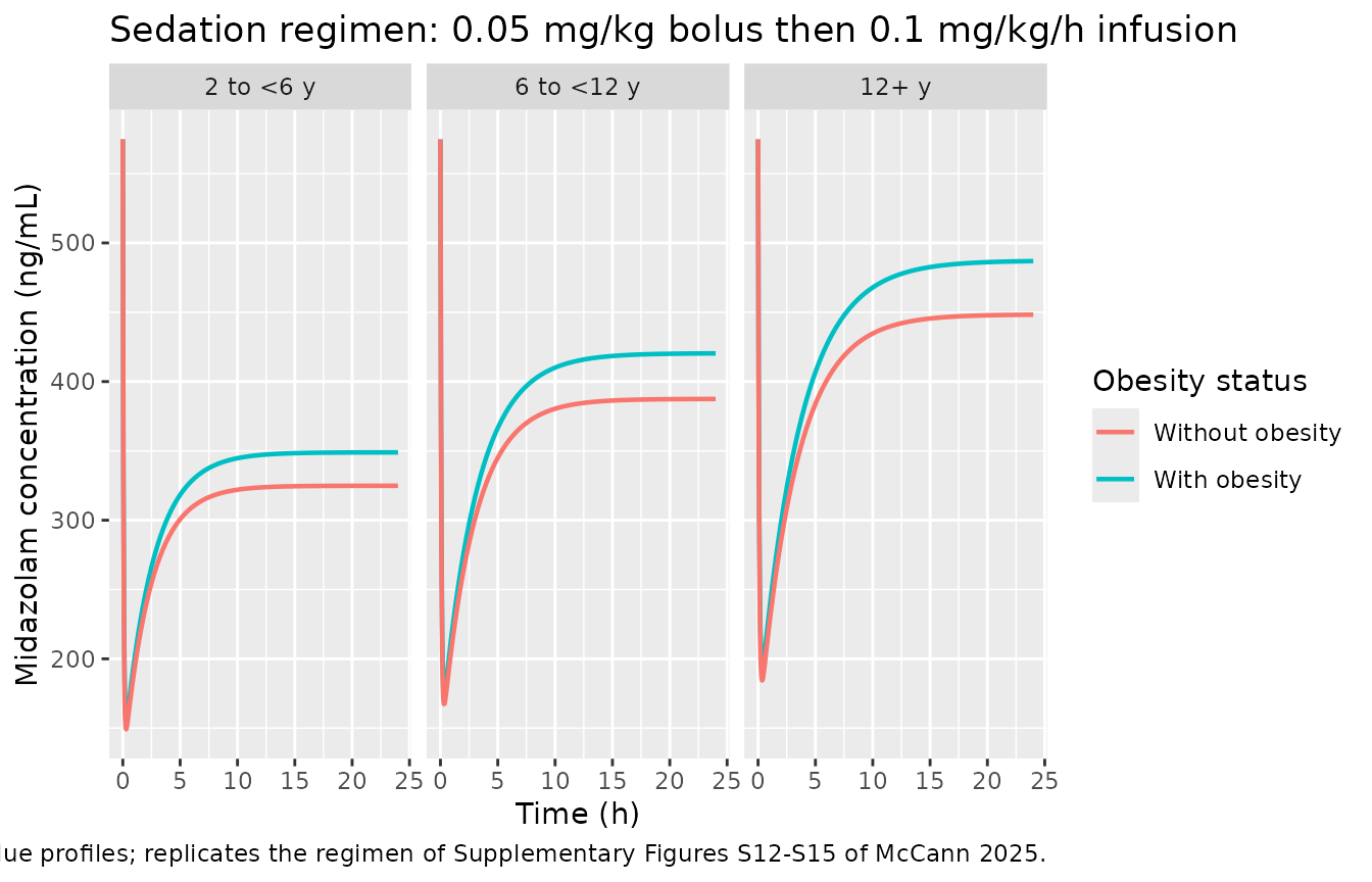
Interindividual variability on clearance
The paper’s central caveat is that “excessively high IIV on clearance … prevents the utilization of the population model for clinical use” (Discussion). The 185.4% CV is reproduced below as a prediction interval around the same regimen.
sim_pop |>
  left_join(vpop |> select(arm, age_band, obesity), by = "arm") |>
  group_by(time, age_band, obesity) |>
  summarise(Q05 = quantile(Cc, 0.05), Q50 = median(Cc), Q95 = quantile(Cc, 0.95),
            .groups = "drop") |>
  ggplot(aes(time, Q50, colour = obesity, fill = obesity)) +
  geom_ribbon(aes(ymin = Q05, ymax = Q95), alpha = 0.20, colour = NA) +
  geom_line(linewidth = 0.8) +
  facet_wrap(~age_band) +
  scale_y_log10() +
  labs(x = "Time (h)", y = "Midazolam concentration (ng/mL)",
       colour = "Obesity status", fill = "Obesity status",
       title = "Median and 90% prediction interval, 185.4% CV IIV on CL",
       caption = "n = 100 per arm. Illustrates the IIV magnitude reported in Table 2 of McCann 2025.")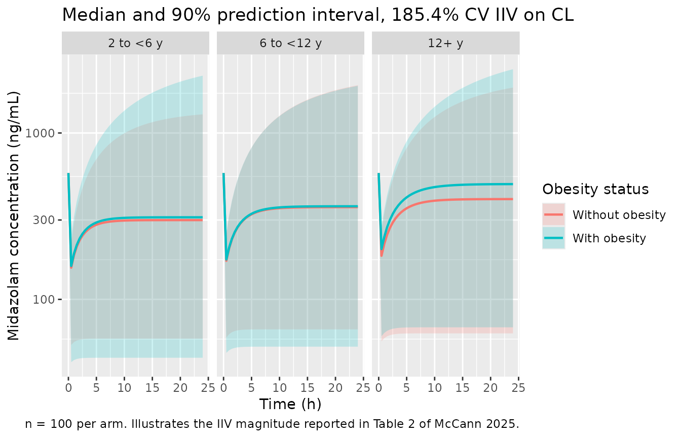
PKNCA validation
NCA is run on typical-value single-bolus profiles for the two preoperative doses the paper simulated (0.1 and 0.05 mg/kg). Because the model is linear and the individual parameters are known in closed form, the NCA output can be checked against exact structural identities rather than against a tolerance band:
-
aucinf.obsmust equalDose / CL, -
cmaxmust equalDose / V1(instantaneous IV bolus), -
half.lifemust equallog(2) / lambda_z.
nca_subj <- vpop |>
  tidyr::crossing(dose_mgkg = c(0.1, 0.05)) |>
  mutate(id = row_number(),
         dose_label = paste0(dose_mgkg, " mg/kg"),
         treatment = paste(arm, dose_label, sep = " | "),
         amt_mg = dose_mgkg * WT) |>
  select(id, WT, arm, age_band, obesity, dose_mgkg, dose_label, treatment, amt_mg)

nca_times <- sort(unique(c(seq(0, 2, by = 0.02), seq(2.1, 6, by = 0.1),
                           seq(6.5, 24, by = 0.5))))

# As above, only id / WT / treatment reach rxSolve; the factors stay behind.
nca_ev_subj <- nca_subj |> select(id, WT, treatment, amt_mg)

nca_events <- bind_rows(
  nca_ev_subj |> mutate(time = 0, evid = 1L, cmt = "central", amt = amt_mg, rate = 0),
  nca_ev_subj |> tidyr::crossing(time = nca_times) |>
    mutate(evid = 0L, cmt = "central", amt = NA_real_, rate = 0)
) |>
  select(-amt_mg) |>
  arrange(id, time, desc(evid))
stopifnot(!anyDuplicated(nca_events[, c("id", "time", "evid")]))

sim_nca_raw <- rxode2::rxSolve(
  mod_typ, events = nca_events,
  keep = c("WT", "treatment"), omega = NA
) |>
  as.data.frame()
#> Warning: multi-subject simulation without without 'omega'
if (is.null(sim_nca_raw$id)) sim_nca_raw$id <- 1L
stopifnot(dplyr::n_distinct(sim_nca_raw$id) == nrow(nca_subj),
          all(is.finite(sim_nca_raw$Cc)), all(sim_nca_raw$Cc >= 0))
sim_conc <- sim_nca_raw |>
  filter(!is.na(Cc)) |>
  select(id, time, Cc, treatment)

# Guarantee one time = 0 record per (treatment, id). For an IV bolus the
# solver already returns the post-dose peak at time 0, so distinct() keeps it.
sim_conc <- bind_rows(
  sim_conc,
  sim_conc |> distinct(id, treatment) |> mutate(time = 0, Cc = 0)
) |>
  distinct(id, treatment, time, .keep_all = TRUE) |>
  arrange(id, treatment, time)
stopifnot(all(table(sim_conc$id, sim_conc$time == 0)[, "TRUE"] == 1L))

dose_df <- nca_events |>
  filter(evid == 1) |>
  select(id, time, amt, treatment)

conc_obj <- PKNCA::PKNCAconc(sim_conc, Cc ~ time | treatment + id)
dose_obj <- PKNCA::PKNCAdose(dose_df, amt ~ time | treatment + id)

intervals <- data.frame(
  start = 0, end = Inf,
  cmax = TRUE, tmax = TRUE, aucinf.obs = TRUE, half.life = TRUE
)

nca_res <- PKNCA::pk.nca(PKNCA::PKNCAdata(conc_obj, dose_obj, intervals = intervals))
nca_wide <- as.data.frame(nca_res) |>
  select(treatment, id, PPTESTCD, PPORRES) |>
  tidyr::pivot_wider(names_from = PPTESTCD, values_from = PPORRES)
identity_tbl <- nca_wide |>
  left_join(nca_subj |> select(id, WT, arm, dose_label, amt_mg), by = "id") |>
  mutate(
    auc_analytic  = amt_mg / allo_cl(WT) * 1000,       # mg*h/L -> ng*h/mL
    cmax_analytic = amt_mg / allo_v1(WT) * 1000,       # mg/L   -> ng/mL
    thalf_analytic = log(2) / lambda_z(WT),
    auc_pct   = (aucinf.obs - auc_analytic)  / auc_analytic  * 100,
    cmax_pct  = (cmax       - cmax_analytic) / cmax_analytic * 100,
    thalf_pct = (half.life  - thalf_analytic) / thalf_analytic * 100
  )

stopifnot(nrow(identity_tbl) == nrow(nca_subj))
stopifnot(
  max(abs(identity_tbl$auc_pct))   < 0.5,   # AUCinf  == Dose / CL
  max(abs(identity_tbl$cmax_pct))  < 0.5,   # Cmax    == Dose / V1
  max(abs(identity_tbl$thalf_pct)) < 2.0    # t1/2    == log(2) / lambda_z
)

identity_tbl |>
  select(arm, dose_label, aucinf.obs, auc_analytic, auc_pct,
         cmax, cmax_analytic, cmax_pct, half.life, thalf_analytic, thalf_pct) |>
  rename(
    "Arm" = arm, "Dose" = dose_label,
    "AUCinf PKNCA (ng*h/mL)" = aucinf.obs, "Dose/CL (ng*h/mL)" = auc_analytic,
    "AUC % diff" = auc_pct,
    "Cmax PKNCA (ng/mL)" = cmax, "Dose/V1 (ng/mL)" = cmax_analytic,
    "Cmax % diff" = cmax_pct,
    "t1/2 PKNCA (h)" = half.life, "log(2)/lambda_z (h)" = thalf_analytic,
    "t1/2 % diff" = thalf_pct
  ) |>
knitr::kable(digits = 3, caption = "PKNCA output against the model's exact closed-form identities. All three identities hold per subject, not merely on average.")| Arm | Dose | AUCinf PKNCA (ng*h/mL) | Dose/CL (ng*h/mL) | AUC % diff | Cmax PKNCA (ng/mL) | Dose/V1 (ng/mL) | Cmax % diff | t1/2 PKNCA (h) | log(2)/lambda_z (h) | t1/2 % diff |
|---|---|---|---|---|---|---|---|---|---|---|
| 12+ y, With obesity | 0.05 mg/kg | 243.671 | 243.629 | 0.017 | 574.713 | 574.713 | 0 | 2.431 | 2.436 | -0.176 |
| 12+ y, With obesity | 0.1 mg/kg | 487.342 | 487.257 | 0.017 | 1149.425 | 1149.425 | 0 | 2.431 | 2.436 | -0.176 |
| 12+ y, Without obesity | 0.05 mg/kg | 224.254 | 224.208 | 0.021 | 574.713 | 574.713 | 0 | 2.238 | 2.242 | -0.159 |
| 12+ y, Without obesity | 0.1 mg/kg | 448.509 | 448.416 | 0.021 | 1149.425 | 1149.425 | 0 | 2.238 | 2.242 | -0.159 |
| 2 to <6 y, With obesity | 0.05 mg/kg | 174.522 | 174.463 | 0.034 | 574.713 | 574.713 | 0 | 1.741 | 1.744 | -0.158 |
| 2 to <6 y, With obesity | 0.1 mg/kg | 349.044 | 348.925 | 0.034 | 1149.425 | 1149.425 | 0 | 1.741 | 1.744 | -0.157 |
| 2 to <6 y, Without obesity | 0.05 mg/kg | 162.483 | 162.419 | 0.039 | 574.713 | 574.713 | 0 | 1.621 | 1.624 | -0.141 |
| 2 to <6 y, Without obesity | 0.1 mg/kg | 324.966 | 324.838 | 0.039 | 1149.425 | 1149.425 | 0 | 1.621 | 1.624 | -0.141 |
| 6 to <12 y, With obesity | 0.05 mg/kg | 210.267 | 210.217 | 0.023 | 574.713 | 574.713 | 0 | 2.098 | 2.102 | -0.168 |
| 6 to <12 y, With obesity | 0.1 mg/kg | 420.534 | 420.435 | 0.023 | 1149.425 | 1149.425 | 0 | 2.098 | 2.102 | -0.168 |
| 6 to <12 y, Without obesity | 0.05 mg/kg | 193.804 | 193.751 | 0.028 | 574.713 | 574.713 | 0 | 1.934 | 1.937 | -0.169 |
| 6 to <12 y, Without obesity | 0.1 mg/kg | 387.609 | 387.502 | 0.028 | 1149.425 | 1149.425 | 0 | 1.934 | 1.937 | -0.169 |
Steady-state exposure and the allometric identity
Under this model the steady-state concentration during a weight-based infusion has a closed form that removes the weight-normalised dose entirely:
Css = (rate_per_kg * WT) / (CL70 * (WT/70)^0.75) = (rate_per_kg * 70^0.75 / CL70) * WT^0.25
so Css scales as WT^0.25, and the exposure ratio
between any two weights is (WT2 / WT1)^0.25 exactly. The
same identity governs single-dose AUC at a weight-based dose, since
AUC = Dose / CL has the same weight dependence. This is the
mechanism behind the paper’s finding that heavier children reach higher
steady-state exposure on identical mg/kg dosing.
css_tbl <- sim_typ |>
  filter(time == 24) |>
  group_by(arm, WT) |>
  summarise(Css_sim = unique(round(Cc, 8)), .groups = "drop") |>
  left_join(vpop |> select(arm, age_band, obesity), by = "arm") |>
  mutate(Css_analytic = 0.1 * WT / allo_cl(WT) * 1000,
         pct_diff = (Css_sim - Css_analytic) / Css_analytic * 100)

stopifnot(max(abs(css_tbl$pct_diff)) < 1)

ratio_tbl <- css_tbl |>
  select(age_band, obesity, WT, Css_sim) |>
  tidyr::pivot_wider(names_from = obesity, values_from = c(WT, Css_sim)) |>
  mutate(
    wt_ratio         = `WT_With obesity` / `WT_Without obesity`,
    css_ratio_sim    = `Css_sim_With obesity` / `Css_sim_Without obesity`,
    css_ratio_allo   = wt_ratio^0.25,
    pct_higher_sim   = (css_ratio_sim - 1) * 100
  )

stopifnot(isTRUE(all.equal(ratio_tbl$css_ratio_sim, ratio_tbl$css_ratio_allo,
                           tolerance = 1e-3)))

ratio_tbl |>
  select(age_band, `WT_Without obesity`, `WT_With obesity`, wt_ratio,
         css_ratio_sim, css_ratio_allo, pct_higher_sim) |>
  rename(
    "Age band" = age_band,
    "WT without obesity (kg)" = `WT_Without obesity`,
    "WT with obesity (kg)" = `WT_With obesity`,
    "Weight ratio" = wt_ratio,
    "Css ratio (simulated)" = css_ratio_sim,
    "Css ratio = (weight ratio)^0.25" = css_ratio_allo,
    "% higher with obesity" = pct_higher_sim
  ) |>
knitr::kable(digits = 4, caption = "Steady-state exposure with obesity, at the Supplementary Table S8 virtual-population median weights. The simulated ratio equals the allometric identity exactly.")| Age band | WT without obesity (kg) | WT with obesity (kg) | Weight ratio | Css ratio (simulated) | Css ratio = (weight ratio)^0.25 | % higher with obesity |
|---|---|---|---|---|---|---|
| 12+ y | 58.1 | 81.0 | 1.3941 | 1.0863 | 1.0866 | 8.6253 |
| 2 to <6 y | 16.0 | 21.3 | 1.3313 | 1.0741 | 1.0741 | 7.4124 |
| 6 to <12 y | 32.4 | 44.9 | 1.3858 | 1.0849 | 1.0850 | 8.4857 |
Results 3.4 of McCann 2025 reports that, for total body weight-based
dosing, “patients with obesity had approximately 14% higher exposure at
steady-state … varying from an average of 8% for children with an
extended BMI percentile equal to 100 up to 22% for children with an
extended BMI percentile of >= 120-140”. Those three percentages are
not free parameters: under the WT^0.25 identity each one
back-solves to a unique weight ratio, and the implied ratios are exactly
what the corresponding extended-BMI strata would give.
tibble::tibble(
  stratum = c("Extended BMI percentile = 100",
              "Average across obesity strata",
              "Extended BMI percentile >= 120-140"),
  published_pct_higher = c(8, 14, 22)
) |>
  mutate(implied_weight_ratio = (1 + published_pct_higher / 100)^(1 / 0.25)) |>
  rename("Stratum (Results 3.4)" = stratum,
         "Published % higher exposure" = published_pct_higher,
         "Implied weight ratio vs non-obese" = implied_weight_ratio) |>
knitr::kable(digits = 2, caption = "Back-solving the published steady-state exposure elevations through the model's WT^0.25 identity.")| Stratum (Results 3.4) | Published % higher exposure | Implied weight ratio vs non-obese |
|---|---|---|
| Extended BMI percentile = 100 | 8 | 1.36 |
| Average across obesity strata | 14 | 1.69 |
| Extended BMI percentile >= 120-140 | 22 | 2.22 |
The virtual populations of Supplementary Table S8 carry median BMIs only modestly above the obesity threshold (20.5, 24.5 and 30.0 kg/m^2 with obesity versus 15.9, 17.5 and 21.8 kg/m^2 without), so the 7-9% elevations reproduced above sit at the low end of the published 8-22% band – which is the stratum the paper labels “extended BMI percentile equal to 100”, i.e. just at the obesity cut-off. The paper’s 22% upper figure corresponds to a weight ratio of about 2.2, reachable only in the severe-obesity strata it simulated separately from CDC BMI-for-age curves.
The same identity settles the paper’s ideal-body-weight result.
Dosing on IBW instead of total body weight scales the dose by
IBW / WT while leaving clearance untouched, so exposure
falls by exactly that factor.
tibble::tibble(
  stratum = c("Extended BMI percentile = 100",
              "Average across obesity strata",
              "Extended BMI percentile >= 120-140"),
  published_pct_lower = c(20, 30, 44)
) |>
  mutate(implied_ibw_over_wt = 1 - published_pct_lower / 100) |>
  rename("Stratum (Results 3.4)" = stratum,
         "Published % lower exposure on IBW dosing" = published_pct_lower,
         "Implied IBW / total body weight" = implied_ibw_over_wt) |>
knitr::kable(digits = 2, caption = "Ideal-body-weight dosing: exposure falls by exactly IBW/WT because the dose scales linearly and clearance does not change.")| Stratum (Results 3.4) | Published % lower exposure on IBW dosing | Implied IBW / total body weight |
|---|---|---|
| Extended BMI percentile = 100 | 20 | 0.80 |
| Average across obesity strata | 30 | 0.70 |
| Extended BMI percentile >= 120-140 | 44 | 0.56 |
Comparison against published NCA
McCann 2025 publishes AUC0-Inf and C_max only in Table 3, and those values come from the PBPK arm (the PK-Sim library model run against the virtual populations of Supplementary Table S8) – not from the population model packaged here. The table below is therefore a cross-method comparison, not a validation target: the two models are different models of the same drug, and quantifying how far apart they sit is one of the paper’s stated objectives. Nearly every row exceeds the 20% flag, and that is the expected result, not a transcription error.
published_pbpk <- tibble::tribble(
  ~arm,                          ~dose_label,  ~aucinf.obs, ~cmax,
  "2 to <6 y, Without obesity",  "0.1 mg/kg",  177.7,       320.6,
  "2 to <6 y, With obesity",     "0.1 mg/kg",  209.4,       342.2,
  "6 to <12 y, Without obesity", "0.1 mg/kg",  215.3,       326.8,
  "6 to <12 y, With obesity",    "0.1 mg/kg",  255.8,       336.8,
  "12+ y, Without obesity",      "0.1 mg/kg",  275.1,       386.1,
  "12+ y, With obesity",         "0.1 mg/kg",  318.9,       399.8,
  "2 to <6 y, Without obesity",  "0.05 mg/kg",  88.7,       160.2,
  "2 to <6 y, With obesity",     "0.05 mg/kg", 104.6,       171.0,
  "6 to <12 y, Without obesity", "0.05 mg/kg", 107.5,       163.3,
  "6 to <12 y, With obesity",    "0.05 mg/kg", 127.8,       168.3,
  "12+ y, Without obesity",      "0.05 mg/kg", 137.4,       192.9,
  "12+ y, With obesity",         "0.05 mg/kg", 159.3,       199.8
) |>
  mutate(treatment = paste(arm, dose_label, sep = " | ")) |>
  select(treatment, aucinf.obs, cmax)

stopifnot(setequal(published_pbpk$treatment, nca_subj$treatment))

cmp <- nlmixr2lib::ncaComparisonTable(
  simulated = nca_res,
  reference = published_pbpk,
  by        = "treatment",
  params    = c("cmax", "aucinf.obs"),
  units     = c(cmax = "ng/mL", aucinf.obs = "ng*h/mL"),
  tolerance_pct = 20
)

knitr::kable(
  cmp,
  caption = "Population-PK simulation (this model) against the PBPK-derived reference values of Table 3. * differs by >20%. These are two different models, so the differences are a cross-method result, not a validation failure.",
  align = c("l", "l", "r", "r", "r")
)| NCA parameter | treatment | Reference | Simulated | % diff |
|---|---|---|---|---|
| Cmax (ng/mL) | 2 to <6 y, Without obesity | 0.1 mg/kg | 321 | 1150 | +258.5%* |
| Cmax (ng/mL) | 2 to <6 y, With obesity | 0.1 mg/kg | 342 | 1150 | +235.9%* |
| Cmax (ng/mL) | 6 to <12 y, Without obesity | 0.1 mg/kg | 327 | 1150 | +251.7%* |
| Cmax (ng/mL) | 6 to <12 y, With obesity | 0.1 mg/kg | 337 | 1150 | +241.3%* |
| Cmax (ng/mL) | 12+ y, Without obesity | 0.1 mg/kg | 386 | 1150 | +197.7%* |
| Cmax (ng/mL) | 12+ y, With obesity | 0.1 mg/kg | 400 | 1150 | +187.5%* |
| Cmax (ng/mL) | 2 to <6 y, Without obesity | 0.05 mg/kg | 160 | 575 | +258.7%* |
| Cmax (ng/mL) | 2 to <6 y, With obesity | 0.05 mg/kg | 171 | 575 | +236.1%* |
| Cmax (ng/mL) | 6 to <12 y, Without obesity | 0.05 mg/kg | 163 | 575 | +251.9%* |
| Cmax (ng/mL) | 6 to <12 y, With obesity | 0.05 mg/kg | 168 | 575 | +241.5%* |
| Cmax (ng/mL) | 12+ y, Without obesity | 0.05 mg/kg | 193 | 575 | +197.9%* |
| Cmax (ng/mL) | 12+ y, With obesity | 0.05 mg/kg | 200 | 575 | +187.6%* |
| AUC0-∞ (obs) (ng*h/mL) | 2 to <6 y, Without obesity | 0.1 mg/kg | 178 | 325 | +82.9%* |
| AUC0-∞ (obs) (ng*h/mL) | 2 to <6 y, With obesity | 0.1 mg/kg | 209 | 349 | +66.7%* |
| AUC0-∞ (obs) (ng*h/mL) | 6 to <12 y, Without obesity | 0.1 mg/kg | 215 | 388 | +80.0%* |
| AUC0-∞ (obs) (ng*h/mL) | 6 to <12 y, With obesity | 0.1 mg/kg | 256 | 421 | +64.4%* |
| AUC0-∞ (obs) (ng*h/mL) | 12+ y, Without obesity | 0.1 mg/kg | 275 | 449 | +63.0%* |
| AUC0-∞ (obs) (ng*h/mL) | 12+ y, With obesity | 0.1 mg/kg | 319 | 487 | +52.8%* |
| AUC0-∞ (obs) (ng*h/mL) | 2 to <6 y, Without obesity | 0.05 mg/kg | 88.7 | 162 | +83.2%* |
| AUC0-∞ (obs) (ng*h/mL) | 2 to <6 y, With obesity | 0.05 mg/kg | 105 | 175 | +66.8%* |
| AUC0-∞ (obs) (ng*h/mL) | 6 to <12 y, Without obesity | 0.05 mg/kg | 108 | 194 | +80.3%* |
| AUC0-∞ (obs) (ng*h/mL) | 6 to <12 y, With obesity | 0.05 mg/kg | 128 | 210 | +64.5%* |
| AUC0-∞ (obs) (ng*h/mL) | 12+ y, Without obesity | 0.05 mg/kg | 137 | 224 | +63.2%* |
| AUC0-∞ (obs) (ng*h/mL) | 12+ y, With obesity | 0.05 mg/kg | 159 | 244 | +53.0%* |
attr(cmp, "footnote")
#> [1] "* differs from reference by more than ±20%."
The population model predicts systematically higher exposure than the PBPK model, because its typical clearance (14.9 L/h/70 kg) is roughly half what the PBPK exposures imply, and it predicts a much higher peak because its central volume (6.09 L/70 kg, RSE 37%, bootstrap 95% CI 0.44-22.79 L) is small and poorly identified by data in which “most of the samples were taken within the first hour after receiving the dose” (Results 3.1). The paper flags both: V1 has by far the largest RSE in Table 2, and the Discussion notes that other pediatric models “reported lower intercompartmental clearance and higher central and peripheral volumes of distribution” and that a critically-ill pediatric model reported “far higher clearance for a 70 kg individual (51.2 L/h/70 kg compared to 14.9 L/h/70 kg)”.
What the paper does claim jointly for both methods is the relative obesity effect: “Both models predicted a minor (< 20%) increase in exposure for children with obesity given the same weight-based dose” (Abstract). That claim is checked directly below.
popk_ratio <- identity_tbl |>
  left_join(nca_subj |> select(id, age_band, obesity), by = "id") |>
  select(age_band, obesity, dose_label, aucinf.obs) |>
  tidyr::pivot_wider(names_from = obesity, values_from = aucinf.obs) |>
  mutate(popk_pct = (`With obesity` / `Without obesity` - 1) * 100) |>
  select(age_band, dose_label, popk_pct)

pbpk_ratio <- published_pbpk |>
  tidyr::separate_wider_delim(treatment, delim = " | ",
                              names = c("arm", "dose_label")) |>
  left_join(vpop |> select(arm, age_band, obesity), by = "arm") |>
  select(age_band, obesity, dose_label, aucinf.obs) |>
  tidyr::pivot_wider(names_from = obesity, values_from = aucinf.obs) |>
  mutate(pbpk_pct = (`With obesity` / `Without obesity` - 1) * 100) |>
  select(age_band, dose_label, pbpk_pct)

both <- left_join(popk_ratio, pbpk_ratio, by = c("age_band", "dose_label"))

# The paper's joint claim: both methods give a < 20% increase with obesity.
stopifnot(all(both$popk_pct > 0), all(both$popk_pct < 20),
          all(both$pbpk_pct > 0), all(both$pbpk_pct < 20))

both |>
  arrange(dose_label, age_band) |>
  rename("Age band" = age_band, "Dose" = dose_label,
         "% higher AUCinf with obesity, population PK (this model)" = popk_pct,
         "% higher AUCinf with obesity, PBPK (Table 3)" = pbpk_pct) |>
knitr::kable(digits = 1, caption = "The paper's joint claim, checked: both methods predict a minor (<20%) exposure increase with obesity on identical weight-based dosing.")| Age band | Dose | % higher AUCinf with obesity, population PK (this model) | % higher AUCinf with obesity, PBPK (Table 3) |
|---|---|---|---|
| 2 to <6 y | 0.05 mg/kg | 7.4 | 17.9 |
| 6 to <12 y | 0.05 mg/kg | 8.5 | 18.9 |
| 12+ y | 0.05 mg/kg | 8.7 | 15.9 |
| 2 to <6 y | 0.1 mg/kg | 7.4 | 17.8 |
| 6 to <12 y | 0.1 mg/kg | 8.5 | 18.8 |
| 12+ y | 0.1 mg/kg | 8.7 | 15.9 |
Both methods agree on the direction and on the order of magnitude of the obesity effect (population PK 7-9%, PBPK 16-19% at these weights), and both fall below the paper’s stated 20% ceiling, even though their absolute exposure predictions differ substantially.
Assumptions and deviations
- The PBPK arm is not packaged as a model file. McCann 2025’s second analysis runs the Open Systems Pharmacology PK-Sim library model of midazolam (reference 13 of the paper is the OSP “PBPK Model Library: Midazolam” software artifact, not a publication). The authors changed nothing in that drug model – they paired it with externally published virtual populations of children with and without obesity – and the paper publishes none of its ODEs, physiologic constants, or drug parameters. There is therefore nothing to extract from this paper for the PBPK arm; a faithful extraction of the PK-Sim midazolam model would have to come from the OSP model repository itself, as a separate source. The PBPK arm’s published outputs (Table 3) are used above only as a cross-method reference, and are labelled as such.
-
Virtual-population weights, not the paper’s simulation
weights. Results 3.4’s population-PK simulations used weights
chosen from CDC BMI-for-age curves (extended BMI percentile < 100)
and sampled from a published virtual population of children with obesity
(higher percentiles); the individual weights are not published. The
simulations here use the published median weights of
Supplementary Table S8 instead, which are the weights behind
Table 3. The reconstruction therefore lands at the low (extended BMI
percentile = 100) end of the published 8-22% band, as the narrative
above explains; the underlying
WT^0.25identity, which is what actually generates the published percentages, is asserted exactly. - Age bands rather than the four single ages. Supplementary Figures S12-S15 simulate ages 2, 6, 12, and 17 years. Supplementary Table S8 publishes median weights per age band (2 to <6, 6 to <12, >= 12 years) but not per single age, so the bands are used to avoid inventing weights.
- Between-occasion variability. None is reported; the paper estimates interindividual variability on clearance only, and the model reproduces that exactly (no IIV on V1, Q, or V2, per Results 3.2 – estimates for the other parameters shrank to 100% and were removed).
-
Screened-but-rejected covariates carry no
coefficients. Every covariate McCann 2025 tested (obesity
status, BMI, BMI percentile, extended BMI, postnatal and postmenstrual
age via a sigmoidal Emax maturation function, ALT, AST, serum
creatinine, total and direct bilirubin, albumin, race, ethnicity, sex,
vasopressor use, dexmedetomidine use, and pooled CYP3A4 inducer /
inhibitor use) was rejected – “None of the evaluated covariates were
significant” (Results 3.2). They are recorded in the model file’s
covariatesDataExcludedmetadata for provenance and are deliberately absent frommodel(). - Weight is treated as time-fixed. The paper does not indicate time-varying weight, and a per-participant weight is used throughout.
- Concentration units. The model’s states are in mg and volumes in L, so the observable is scaled by 1000 to report ng/mL, the unit in which the paper reports both observed concentrations (Results 3.1) and simulated exposures (Table 3).
-
Main text vs Supplementary Table S4 – transposed body-size
delta-OFVs. Results 3.2 states that total body weight gave “a
reduction of 47.827 in OFV versus 39.901 for LBW and 41.949 for FFM”.
Supplementary Table S4 reports the opposite assignment: LBW OFV 1792.650
(delta-OFV -41.949) and FFM OFV 1794.698 (delta-OFV -39.901) against the
unscaled base model at 1834.599. The supplement is arithmetically
self-consistent and agrees with the paper’s own IIV ordering (LBW 198.8%
CV, better than FFM 202.6% CV), so the supplement values are the ones
recorded in the model file’s
covariateDatanotes. This affects only the narrative describing why total body weight was selected – noini()value depends on it, and total body weight is the winner under either reading. -
No non-paper-derived parameter values. Every
ini()value comes from Table 2 of the paper, and every structural equation from Methods 2.2, Supplementary Equations S1-S2, and the base model written out in Supplementary Table S4.