Trontinemab and gantenerumab PK in plasma and brain (Grimm 2023)
Source:vignettes/articles/Grimm_2023.Rmd
Grimm_2023.Rmd
library(nlmixr2lib)
library(dplyr)
#>
#> Attaching package: 'dplyr'
#> The following objects are masked from 'package:stats':
#>
#>     filter, lag
#> The following objects are masked from 'package:base':
#>
#>     intersect, setdiff, setequal, union
library(ggplot2)
Model and source
- Citation: Grimm HP, Schumacher V, Schafer M, et al. Delivery of the Brainshuttle amyloid-beta antibody fusion trontinemab to non-human primate brain and projected efficacious dose regimens in humans. mAbs. 2023;15(1):2261509. doi:10.1080/19420862.2023.2261509
- Description (trontinemab): Trontinemab PK model in non-human primates (Grimm 2023): two-compartment plasma PK with Michaelis-Menten elimination and brain-region effect-compartment distribution (brain_cerebellum, brain_hippocampus, brain_striatum, brain_cortex, choroid plexus, CSF).
- Description (gantenerumab): Gantenerumab PK model in cynomolgus monkeys (Grimm 2023): two-compartment plasma PK with brain extracellular distribution across six brain regions (brain_cerebellum, brain_hippocampus, brain_striatum, brain_cortex, choroid plexus, CSF).
- Article: https://doi.org/10.1080/19420862.2023.2261509
Trontinemab replication
Simulate trontinemab PK in plasma and brain
Replicate figures 2 and 3 in the publication with a single 10 mg/kg dose to a cynomolgus monkey.
dSimDose <-
  data.frame(
    ID = 1,
    AMT = 10, # dose in mg/kg # nolint: commented_code_linter.
    WT = 5, # cynomologus monkey body weight according to the paper
    TIME = 0,
    EVID = 1,
    CMT = "central"
  )
dSimObs <-
  data.frame(
    ID = 1,
    AMT = 0,
    WT = 5,
    TIME = c(5 / 60, 1, 2, 4, 8, 12, seq(24, 336, by = 24)),
    EVID = 0,
    CMT = "central"
  )
dSimPrep <- dplyr::bind_rows(dSimDose, dSimObs)
Grimm2023Tront <- readModelDb("Grimm_2023_trontinemab")
conc_unit <- rxode2::rxode(Grimm2023Tront)$units[["concentration"]]
#> ℹ parameter labels from comments will be replaced by 'label()'
# Set BSV to zero for simulation to get a reproducible result
dSimTront <- rxode2::rxSolve(Grimm2023Tront |> rxode2::zeroRe(), events = dSimPrep)
#> ℹ parameter labels from comments will be replaced by 'label()'
#> ℹ omega/sigma items treated as zero: 'etalfpla_cerebellum', 'etalfpla_hippocampus', 'etalfpla_striatum', 'etalfpla_cortex', 'etalfpla_choroid_plexus'
dSimTront$Analyte <- "Trontinemab"
Simulate gantenerumab PK in plasma and brain
Replicate figures 2 and 3 in the publication with a single 20 mg/kg dose to a cynomolgus monkey.
dSimDose <-
  data.frame(
    ID = 1,
    AMT = 20, # dose in mg/kg # nolint: commented_code_linter.
    WT = 5, # cynomologus monkey body weight according to the paper
    TIME = 0,
    EVID = 1,
    CMT = "central"
  )
dSimObs <-
  data.frame(
    ID = 1,
    AMT = 0,
    WT = 5,
    TIME = c(5 / 60, 1, 2, 4, 8, 12, seq(24, 336, by = 24)),
    EVID = 0,
    CMT = "central"
  )
dSimPrep <- dplyr::bind_rows(dSimDose, dSimObs)
Grimm2023Gant <- readModelDb("Grimm_2023_gantenerumab")
# Set BSV to zero for simulation to get a reproducible result
dSimGant <- rxode2::rxSolve(Grimm2023Gant |> rxode2::zeroRe(), events = dSimPrep)
#> ℹ omega/sigma items treated as zero: 'etalfpla_cerebellum', 'etalfpla_hippocampus', 'etalfpla_striatum', 'etalfpla_cortex', 'etalfpla_choroid_plexus'
dSimGant$Analyte <- "Gantenerumab"
Plot plasma PK
Replicate figure 2 from the paper.
dSim <- bind_rows(dSimTront, dSimGant)
dSim$Analyte <- factor(dSim$Analyte, levels = c("Trontinemab", "Gantenerumab"))

ggplot(dSim, aes(x = time, y = sim)) +
  geom_line() +
  labs(
    x = "Time (h)",
    y = paste0("Concentration (", conc_unit, ")")
  ) +
  scale_y_log10() +
  scale_x_continuous(breaks = seq(0, 336, by = 48)) +
  coord_cartesian(ylim = c(1e3, NA)) +
  facet_grid(~Analyte)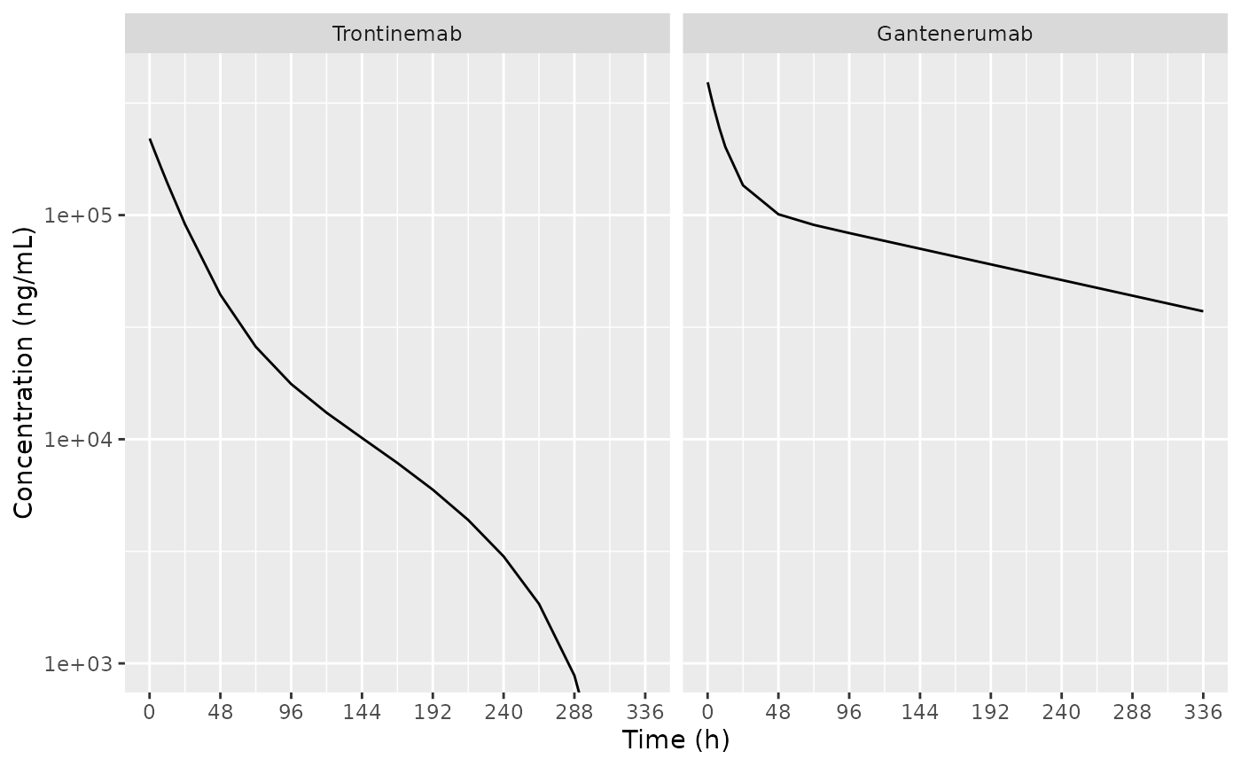
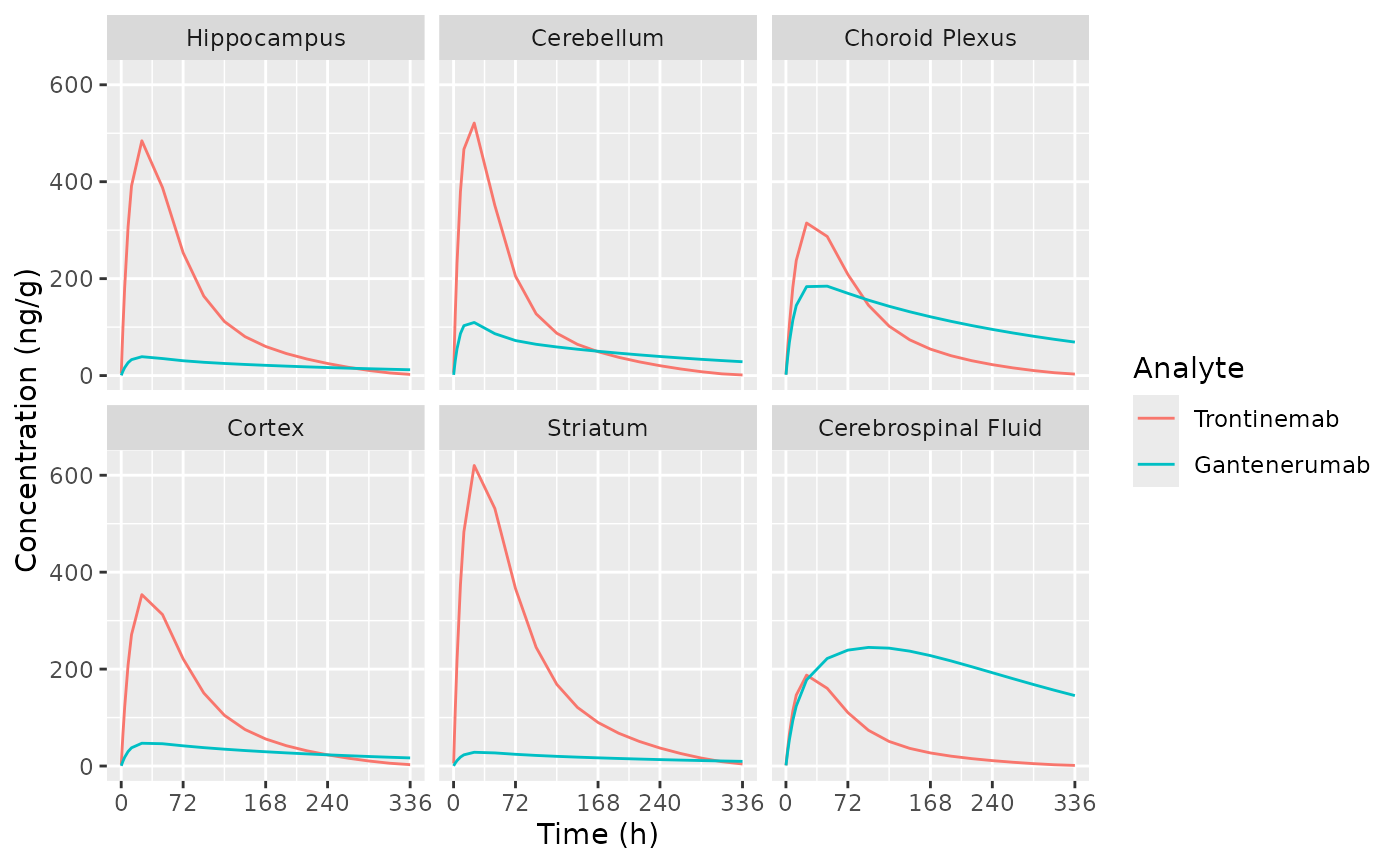
Plot brain PK
Replicate figure 3 from the paper.
d_plot_brain <-
  dSim |>
  select(
    time, Analyte,
    any_of(c("cerebellum", "hippocampus", "striatum", "cortex",
             "choroid_plexus", "csf"))
  ) |>
  tidyr::pivot_longer(cols = -c("time", "Analyte"), names_to = "ASPEC", values_to = "AVAL") |>
  mutate(
    ASPEC =
      factor(
        ASPEC,
        levels = c("hippocampus", "cerebellum", "choroid_plexus", "cortex", "striatum", "csf"),
        labels = c("Hippocampus", "Cerebellum", "Choroid Plexus", "Cortex", "Striatum", "Cerebrospinal Fluid")
      )
  )

ggplot(d_plot_brain, aes(x = time, y = AVAL, colour = Analyte)) +
  geom_line() +
  labs(
    x = "Time (h)",
    y = "Concentration (ng/g)"
  ) +
  scale_x_continuous(breaks = c(0, 72, 168, 240, 336)) +
  facet_wrap(~ASPEC)