Doxorubicin + dexrazoxane in breast cancer cells (Mody 2023) • nlmixr2lib

Model and source

Article: https://doi.org/10.3389/fphar.2023.1239141 (Front Pharmacol 14:1239141, PMC10620511)
Companion paper supplying the clinical plasma PK and the medium-degradation equations: https://doi.org/10.1038/s41598-023-29964-4 (Sci Rep 13:3100, PMC9947016), packaged separately as Mody_2023_doxorubicin_dexrazoxane.

Mody and co-workers characterised the anticancer effects of doxorubicin (DOX) and its cardioprotectant dexrazoxane (DEX) in two “difficult-to-treat” breast cancer cell lines, and then translated the resulting cell-based pharmacodynamic (PD) models to a clinically relevant dosing regimen. The paper reports three model layers, each fitted separately per cell line, so the extraction is six model files sharing this one vignette.

Model file	Layer	Cell line	Source
`Mody_2023_doxorubicin_dexrazoxane_static_jimt1`	A: static 72 h concentration-response	JIMT-1	Eqs 1-2, Table 1
`Mody_2023_doxorubicin_dexrazoxane_static_mdamb468`	A	MDA-MB-468	Eqs 1-2, Table 1
`Mody_2023_doxorubicin_dexrazoxane_jimt1`	B: cellular PD time course	JIMT-1	Eqs 3, 3a-3e, 4a-4i, Table 2
`Mody_2023_doxorubicin_dexrazoxane_mdamb468`	B	MDA-MB-468	Eqs 3, 3a-3e, 4a-4i, Table 2
`Mody_2023_doxorubicin_dexrazoxane_clinical_jimt1`	C: clinical translation	JIMT-1	Methods + Figure 6
`Mody_2023_doxorubicin_dexrazoxane_clinical_mdamb468`	C	MDA-MB-468	Methods + Figure 6

# readModelDb() returns the model *function*, which has no $theta / $iniDf.
# Resolve each one to its rxUi here so the parameter accessors below work.
load_ui <- function(nm) rxode2::rxode(readModelDb(nm))

mA <- list(
  jimt1    = load_ui("Mody_2023_doxorubicin_dexrazoxane_static_jimt1"),
  mdamb468 = load_ui("Mody_2023_doxorubicin_dexrazoxane_static_mdamb468")
)
mB <- list(
  jimt1    = load_ui("Mody_2023_doxorubicin_dexrazoxane_jimt1"),
  mdamb468 = load_ui("Mody_2023_doxorubicin_dexrazoxane_mdamb468")
)
mC <- list(
  jimt1    = load_ui("Mody_2023_doxorubicin_dexrazoxane_clinical_jimt1"),
  mdamb468 = load_ui("Mody_2023_doxorubicin_dexrazoxane_clinical_mdamb468")
)
cell_label <- c(jimt1 = "JIMT-1", mdamb468 = "MDA-MB-468")

Population

There is no human study population behind Layers A and B: the data are in-vitro CCK-8 cell-viability assays in two human breast cancer cell lines chosen as prototypes for difficult-to-treat disease. JIMT-1 is HER2-expressing but trastuzumab-resistant; MDA-MB-468 is triple-negative. JIMT-1 cells were seeded at 3 x 10^3 and MDA-MB-468 at 5 x 10^3 cells per 100 uL well of a 96-well plate, incubated overnight, then exposed to DOX (0.005-1 uM), DEX (6.25-200 uM) or one of 36 DOX x DEX combinations for 72-96 h. Each condition was run in at least triplicate against matched vehicle controls.

Layer C projects those cell models onto a simulated typical adult cancer patient with a body surface area of 1.8 m^2, receiving DOX 50 mg/m^2 (90 mg) every three weeks as a 15-min IV infusion, alone or with DEX 500 mg/m^2 (900 mg) – the 10:1 DEX:DOX ratio the companion paper identified as maximally cardioprotective – for three cycles.

The same information is available programmatically, e.g. readModelDb("Mody_2023_doxorubicin_dexrazoxane_jimt1")()$population.

Source trace

Per-parameter provenance is recorded as an in-file comment beside every ini() entry. Collected here for review:

Equation / parameter	Value (JIMT-1 / MDA-MB-468)	Source location
`R = R0(1 - ImaxC/(IC50 + C))`	n/a	Eq 1
Competitive interaction model	n/a	Eq 2
`limax_dox`	0.988 / 0.959	Table 1
`lec50_dox`	214 nM = 0.214 uM / 21.1 nM = 0.0211 uM	Table 1
`limax_dexrazoxane`	0.74 / 0.825	Table 1
`lec50_dexrazoxane`	97.5 uM / 36 uM	Table 1
`lpsi` (Layer A)	1.11 / 0.84	Results, Figure 2 caption
`lhill_dox`, `lhill_dexrazoxane`	1 / 1 (fixed)	not reported; Eq 1 carries no Hill exponent
`dC/dt = -kdeg*C`	n/a	Companion Sci Rep Eqs 1-2
`lkdeg_dox`	0.022 1/h (fixed)	Results, “Time course effects”
`lkdeg_dexrazoxane`	0.054 1/h (fixed)	Results, “Time course effects”
`dR/dt = kg*R`	n/a	Eq 3
`lrbase`	100 % (fixed)	Table 2
`lkgrow`	0.0171 / 0.0167 1/h	Table 2
`lkmax_dox` (Smax,DOX)	0.0705 / 1.16 1/h	Table 2
`lkc50_dox` (SC50,DOX)	0.315 / 0.761 uM	Table 2
`lktr_dox` (1/tau_DOX)	0.0703 / 0.0275 1/h	Table 2
`lkmax_dexrazoxane`	0.0482 / 0.29 1/h	Table 2
`lkc50_dexrazoxane`	21.2 / 17.5 uM	Table 2
`lktr_dexrazoxane`	0.0335 / 0.0182 1/h	Table 2
`lpsi` (Layer B)	~2 / ~1	Table 2
Transit chain, kill function, Eq 4i	n/a	Eqs 3a-3e (single agent), 4a-4i (combination)
`lcl_dox`, `lvc_dox`, `lq_dox`, `lvp_dox`, `lq2_dox`, `lvp2_dox`	53.3 L/h, 17.7 L, 58.7 L/h, 1830 L, 21.8 L/h, 71.6 L	Companion Sci Rep Table 2 (top)
`lkel_dexrazoxane`, `lk12_dexrazoxane`, `lk21_dexrazoxane`, `lvc_dexrazoxane`	1, 1, 1 1/h, 14.6 L	Companion Sci Rep Table 2 (bottom)
`lkp_tumor_dox` (Fac1)	57.1 (fixed)	Results, “Optimization of DOX and DEX combinations”
`lkp_tumor_dexrazoxane` (Fac2)	1 (fixed; arbitrary, paper simulates 0.1/1/10)	Methods
`lconv_dox`, `lconv_dexrazoxane`	1.8397, 3.7275	not from the paper – literature molar masses (see Assumptions)

Layer A: static 72-hour concentration-response

Layer A is algebraic, not dynamic: it maps the two nominal applied concentrations onto percent viability at the 72 h endpoint. The two concentrations enter as covariates.

static_predict <- function(model, dox, dex, psi = NULL) {
  if (!is.null(psi)) model <- rxode2::ini(model, lpsi = log(psi))
  ev <- data.frame(
    id = seq_along(dox), time = 0, evid = 0, amt = NA_real_,
    CONC_DOXORUBICIN = dox, CONC_DEXRAZOXANE = dex
  )
  out <- rxode2::rxSolve(model, ev, returnType = "data.frame")
  # rxSolve omits the `id` column entirely when the event table has a single
  # subject. match() against a NULL column then yields NA and this function
  # silently returns an all-NA prediction, which reads as a failed gate rather
  # than a broken accessor. Fall back to event order, and check the row count
  # rather than assuming it.
  if (is.null(out$id)) {
    stopifnot(nrow(out) == length(dox))
    return(out$viability)
  }
  idx <- match(seq_along(dox), out$id)
  stopifnot(!anyNA(idx))
  out$viability[idx]
}

Gate A1 – the model reproduces the published IC50 by construction

At C_DOX = IC50 with no DEX and an additive interaction (psi = 1), Eq 2 must collapse to Eq 1 and return exactly R0 * (1 - Imax/2).

gateA1 <- lapply(names(mA), function(k) {
  ic50 <- exp(mA[[k]]$theta[["lec50_dox"]])
  imax <- exp(mA[[k]]$theta[["limax_dox"]])
  tibble(
    `Cell line` = cell_label[[k]],
    `IC50 (uM)` = ic50,
    Predicted   = static_predict(mA[[k]], ic50, 0, psi = 1),
    Expected    = 100 * (1 - imax / 2)
  )
}) |> bind_rows() |> mutate(`Abs. difference` = abs(Predicted - Expected))
#> ℹ change initial estimate of `lpsi` to `0`
#> ℹ change initial estimate of `lpsi` to `0`

knitr::kable(gateA1, digits = 6,
             caption = "Gate A1: Eq 2 collapses to Eq 1 at the published IC50.")

Gate A1: Eq 2 collapses to Eq 1 at the published IC50.
Cell line	IC50 (uM)	Predicted	Expected	Abs. difference
JIMT-1	0.2140	50.60	50.60	0
MDA-MB-468	0.0211	52.05	52.05	0

stopifnot(all(gateA1$`Abs. difference` < 1e-6))

Replicating Figure 2B – the additive response surface

Figure 2B plots the additive (psi = 1) response surface for each cell line with the observed combination data overlaid. The observed data are not published in machine-readable form, so only the surfaces are reproduced here.

dox_lv <- c(0.005, 0.01, 0.05, 0.1, 0.5, 1)
dex_lv <- c(6.25, 12.5, 25, 50, 100, 200)
surf <- expand_grid(cell = names(mA), dox = dox_lv, dex = dex_lv) |>
  group_by(cell) |>
  mutate(viability = static_predict(mA[[cur_group()$cell]], dox, dex, psi = 1)) |>
  ungroup() |>
  mutate(`Cell line` = cell_label[cell])
#> ℹ change initial estimate of `lpsi` to `0`
#> ℹ change initial estimate of `lpsi` to `0`
#> Warning: There were 2 warnings in `mutate()`.
#> The first warning was:
#> ℹ In argument: `viability = static_predict(mA[[cur_group()$cell]], dox, dex,
#>   psi = 1)`.
#> ℹ In group 1: `cell = "jimt1"`.
#> Caused by warning:
#> ! multi-subject simulation without without 'omega'
#> ℹ Run `dplyr::last_dplyr_warnings()` to see the 1 remaining warning.

ggplot(surf, aes(factor(dox), viability, colour = factor(dex), group = factor(dex))) +
  geom_line() + geom_point(size = 1) +
  facet_wrap(~`Cell line`) +
  labs(x = "DOX (uM)", y = "Cell viability (%)", colour = "DEX (uM)",
       title = "Figure 2B -- additive (psi = 1) response surface",
       caption = "Replicates the additive surface of Figure 2B of Mody 2023.")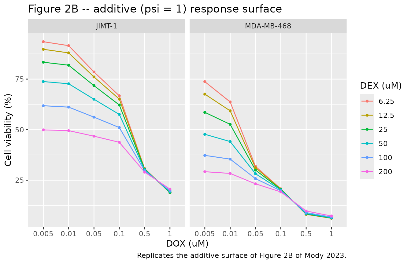

The estimated interaction is modest and points in opposite directions

psiA <- tibble(
  `Cell line`  = unname(cell_label[names(mA)]),
  psi          = vapply(mA, function(m) exp(m$theta[["lpsi"]]), numeric(1)),
  Interpretation = c("modestly antagonistic", "modestly synergistic")
)
knitr::kable(psiA, digits = 3,
             caption = "Layer A interaction parameter (Results / Figure 2 caption).")

Layer A interaction parameter (Results / Figure 2 caption).
Cell line	psi	Interpretation
JIMT-1	1.11	modestly antagonistic
MDA-MB-468	0.84	modestly synergistic

Layer B: cellular PD time course

run_B <- function(model, dox = 0, dex = 0, psi = NULL, tmax = 96, by = 2) {
  if (!is.null(psi)) model <- rxode2::ini(model, lpsi = log(psi))
  ev <- rxode2::et(amt = dox, cmt = "conc_dox") |>
    rxode2::et(amt = dex, cmt = "conc_dexrazoxane") |>
    rxode2::et(seq(0, tmax, by = by))
  rxode2::rxSolve(model, ev, returnType = "data.frame")
}

Gate B1 – the untreated control is pure exponential growth

With no drug, Eq 4i reduces to Eq 3, whose closed-form solution is R(t) = R0 * exp(kg * t).

gateB1 <- lapply(names(mB), function(k) {
  s  <- run_B(mB[[k]])
  kg <- exp(mB[[k]]$theta[["lkgrow"]])
  tibble(`Cell line` = cell_label[[k]],
         `Max relative error` = max(abs(s$viability - 100 * exp(kg * s$time)) /
                                      (100 * exp(kg * s$time))))
}) |> bind_rows()

knitr::kable(gateB1, digits = 10,
             caption = "Gate B1: simulated control vs the analytic exponential solution.")

Gate B1: simulated control vs the analytic exponential solution.
Cell line	Max relative error
JIMT-1	6.658e-07
MDA-MB-468	7.179e-07

stopifnot(all(gateB1$`Max relative error` < 1e-4))

Gate B2 – the transit chain converges on its driving signal

Under a sustained stimulus the three-compartment chain must satisfy K3 -> K once t >> 3*tau. Degradation is switched off for this gate so the stimulus is genuinely constant.

gateB2 <- lapply(names(mB), function(k) {
  m <- rxode2::ini(mB[[k]], lkdeg_dox = log(1e-8), lpsi = log(1))
  s <- run_B(m, dox = 1, tmax = 3000, by = 10)
  kmax <- exp(m$theta[["lkmax_dox"]]); kc50 <- exp(m$theta[["lkc50_dox"]])
  tibble(`Cell line` = cell_label[[k]],
         `K3 at 3000 h` = tail(s$transit3_dox, 1),
         `Driving K`    = kmax * 1 / (kc50 + 1))
}) |> bind_rows() |>
  mutate(`Relative difference` = abs(`K3 at 3000 h` - `Driving K`) / `Driving K`)
#> ℹ change initial estimate of `lkdeg_dox` to `-18.4206807439524`
#> ℹ change initial estimate of `lpsi` to `0`
#> ℹ change initial estimate of `lkdeg_dox` to `-18.4206807439524`
#> ℹ change initial estimate of `lpsi` to `0`

knitr::kable(gateB2, digits = 6,
             caption = "Gate B2: terminal transit compartment approaches the Hill kill rate.")

Gate B2: terminal transit compartment approaches the Hill kill rate.
Cell line	K3 at 3000 h	Driving K	Relative difference
JIMT-1	0.053612	0.053612	7.0e-06
MDA-MB-468	0.658708	0.658717	1.2e-05

stopifnot(all(gateB2$`Relative difference` < 0.01))

Replicating Figures 4B and 4C – single-agent time courses

The single-agent arms correspond to Eqs 3a-3e, i.e. the combination model with psi = 1.

single <- bind_rows(
  expand_grid(cell = names(mB), conc = dox_lv) |> mutate(drug = "DOX"),
  expand_grid(cell = names(mB), conc = dex_lv) |> mutate(drug = "DEX")
) |>
  rowwise() |>
  mutate(sim = list(
    run_B(mB[[cell]],
          dox = if (drug == "DOX") conc else 0,
          dex = if (drug == "DEX") conc else 0,
          psi = 1) |> select(time, viability)
  )) |>
  ungroup() |> tidyr::unnest(sim) |>
  mutate(`Cell line` = cell_label[cell])
#> ℹ change initial estimate of `lpsi` to `0`
#> ℹ change initial estimate of `lpsi` to `0`
#> ℹ change initial estimate of `lpsi` to `0`
#> ℹ change initial estimate of `lpsi` to `0`
#> ℹ change initial estimate of `lpsi` to `0`
#> ℹ change initial estimate of `lpsi` to `0`
#> ℹ change initial estimate of `lpsi` to `0`
#> ℹ change initial estimate of `lpsi` to `0`
#> ℹ change initial estimate of `lpsi` to `0`
#> ℹ change initial estimate of `lpsi` to `0`
#> ℹ change initial estimate of `lpsi` to `0`
#> ℹ change initial estimate of `lpsi` to `0`
#> ℹ change initial estimate of `lpsi` to `0`
#> ℹ change initial estimate of `lpsi` to `0`
#> ℹ change initial estimate of `lpsi` to `0`
#> ℹ change initial estimate of `lpsi` to `0`
#> ℹ change initial estimate of `lpsi` to `0`
#> ℹ change initial estimate of `lpsi` to `0`
#> ℹ change initial estimate of `lpsi` to `0`
#> ℹ change initial estimate of `lpsi` to `0`
#> ℹ change initial estimate of `lpsi` to `0`
#> ℹ change initial estimate of `lpsi` to `0`
#> ℹ change initial estimate of `lpsi` to `0`
#> ℹ change initial estimate of `lpsi` to `0`

control <- expand_grid(cell = names(mB)) |>
  rowwise() |>
  mutate(sim = list(run_B(mB[[cell]]) |> select(time, viability))) |>
  ungroup() |> tidyr::unnest(sim) |> mutate(`Cell line` = cell_label[cell])

ggplot(single, aes(time, viability, colour = factor(conc))) +
  geom_line() +
  geom_line(data = control, aes(time, viability), colour = "black",
            linetype = "dashed", inherit.aes = FALSE) +
  facet_grid(drug ~ `Cell line`) +
  labs(x = "Time (h)", y = "Cell viability (%)", colour = "Conc. (uM)",
       title = "Figures 4B / 4C -- single-agent time courses",
       caption = paste("Replicates Figures 4B and 4C of Mody 2023.",
                       "Dashed black line is the untreated control."))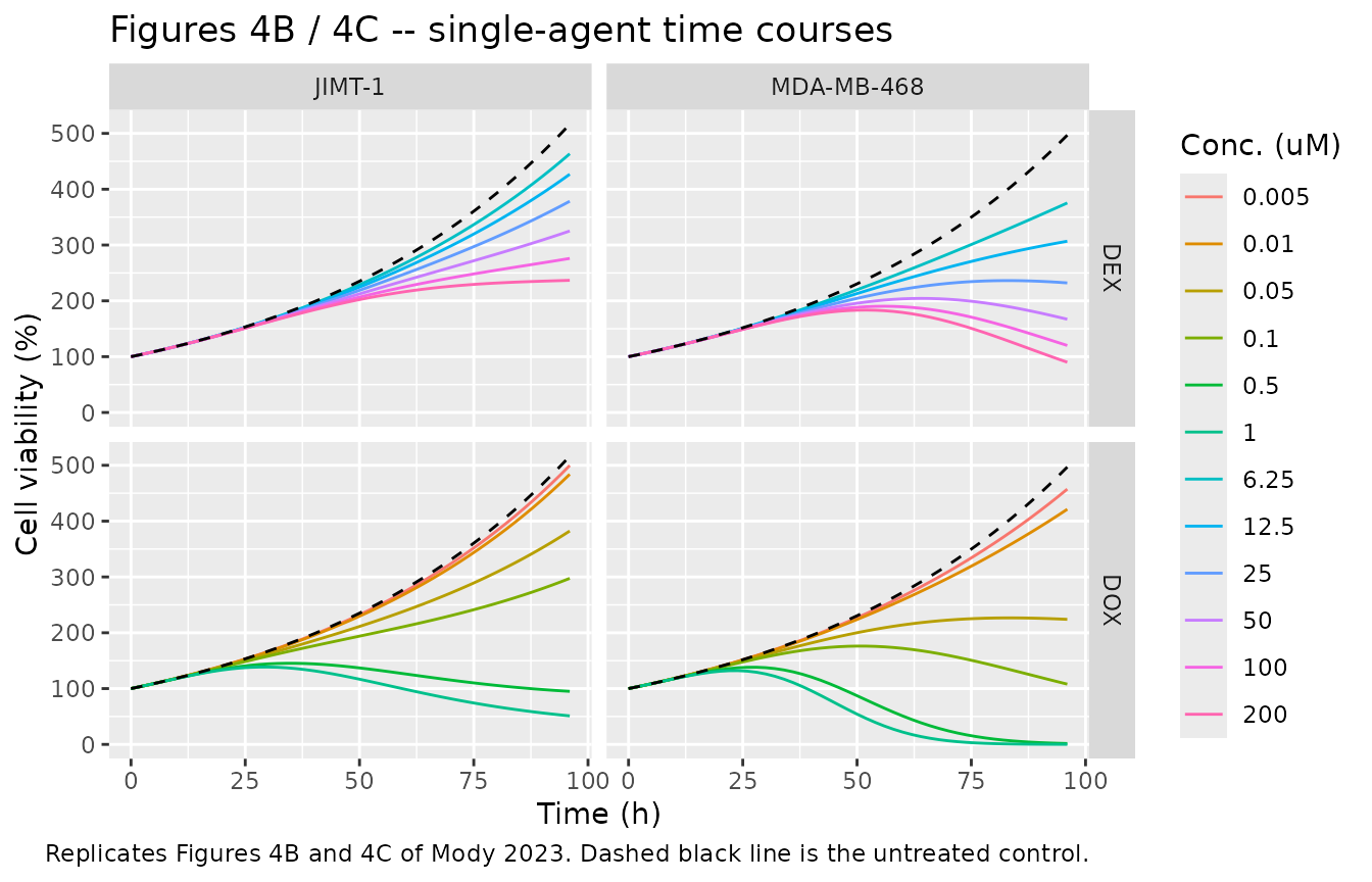

Replicating Figure 5 – combination versus single agents

Here the fitted interaction parameter is in force: psi = 2 (antagonistic) for JIMT-1 and psi = 1 (additive) for MDA-MB-468.

combo <- expand_grid(cell = names(mB), dox = c(0.05, 0.5), dex = c(25, 100)) |>
  rowwise() |>
  mutate(
    Combination = list(run_B(mB[[cell]], dox = dox, dex = dex) |> select(time, viability)),
    `DOX alone` = list(run_B(mB[[cell]], dox = dox, psi = 1) |> select(time, viability)),
    `DEX alone` = list(run_B(mB[[cell]], dex = dex, psi = 1) |> select(time, viability))
  ) |>
  ungroup() |>
  pivot_longer(c(Combination, `DOX alone`, `DEX alone`), names_to = "arm", values_to = "sim") |>
  tidyr::unnest(sim) |>
  mutate(`Cell line` = cell_label[cell],
         panel = paste0("DOX ", dox, " uM + DEX ", dex, " uM"))
#> ℹ change initial estimate of `lpsi` to `0`
#> ℹ change initial estimate of `lpsi` to `0`
#> ℹ change initial estimate of `lpsi` to `0`
#> ℹ change initial estimate of `lpsi` to `0`
#> ℹ change initial estimate of `lpsi` to `0`
#> ℹ change initial estimate of `lpsi` to `0`
#> ℹ change initial estimate of `lpsi` to `0`
#> ℹ change initial estimate of `lpsi` to `0`
#> ℹ change initial estimate of `lpsi` to `0`
#> ℹ change initial estimate of `lpsi` to `0`
#> ℹ change initial estimate of `lpsi` to `0`
#> ℹ change initial estimate of `lpsi` to `0`
#> ℹ change initial estimate of `lpsi` to `0`
#> ℹ change initial estimate of `lpsi` to `0`
#> ℹ change initial estimate of `lpsi` to `0`
#> ℹ change initial estimate of `lpsi` to `0`

ggplot(combo, aes(time, viability, colour = arm)) +
  geom_line() +
  facet_grid(`Cell line` ~ panel, scales = "free_y") +
  labs(x = "Time (h)", y = "Cell viability (%)", colour = NULL,
       title = "Figure 5 -- combination versus single agents",
       caption = "Replicates Figure 5 of Mody 2023.")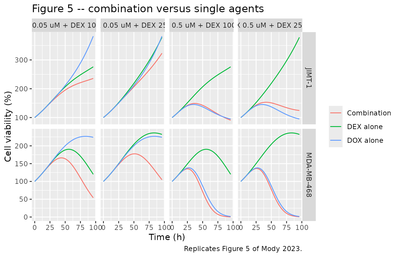

Layer C: in vitro to clinical translation

Layer C drives the same PD model with tumour-site concentrations obtained by scaling the simulated plasma profiles. The models declare three endpoints (plasma DOX, plasma DEX, viability), so observation records must name the compartment they belong to.

dose_ev <- function(with_dex, obs_cmt, tobs) {
  e <- rxode2::et(amt = 90, cmt = "central_dox", dur = 0.25, ii = 504, addl = 2)
  if (with_dex) {
    e <- rxode2::et(e, amt = 900, cmt = "central_dexrazoxane", dur = 0.25, ii = 504, addl = 2)
  }
  rxode2::et(e, tobs, cmt = obs_cmt)
}

Plasma pharmacokinetics and PKNCA validation

# Tmax is 0.25 h, so a 0.25 h grid puts the peak at the very first post-dose
# sample and the trapezoidal AUC below understates AUCinf by ~4.6%. Resolve the
# distribution phase finely enough that the NCA below reproduces Dose/CL to
# within a rounding error rather than within a few percent.
pk_tobs <- sort(unique(c(seq(0, 2, by = 0.005), seq(2, 24, by = 0.05),
                         seq(24, 504, by = 1))))
mC_typ  <- rxode2::zeroRe(mC$jimt1)

pk_dox <- rxode2::rxSolve(mC_typ, dose_ev(TRUE, "Cc_dox", pk_tobs),
                          returnType = "data.frame") |>
  transmute(id = 1L, time, Cc = Cc_dox, treatment = "DOX 90 mg")
#> ℹ omega/sigma items treated as zero: 'etalkgrow', 'etalkmax_dox', 'etalkc50_dox', 'etalktr_dox', 'etalkmax_dexrazoxane', 'etalkc50_dexrazoxane', 'etalktr_dexrazoxane', 'etalpsi', 'etalkp_tumor_dox', 'etalkp_tumor_dexrazoxane'
pk_dex <- rxode2::rxSolve(mC_typ, dose_ev(TRUE, "Cc_dexrazoxane", pk_tobs),
                          returnType = "data.frame") |>
  transmute(id = 1L, time, Cc = Cc_dexrazoxane, treatment = "DEX 900 mg")
#> ℹ omega/sigma items treated as zero: 'etalkgrow', 'etalkmax_dox', 'etalkc50_dox', 'etalktr_dox', 'etalkmax_dexrazoxane', 'etalkc50_dexrazoxane', 'etalktr_dexrazoxane', 'etalpsi', 'etalkp_tumor_dox', 'etalkp_tumor_dexrazoxane'

ggplot(bind_rows(pk_dox, pk_dex), aes(time, Cc)) +
  geom_line() + facet_wrap(~treatment, scales = "free_y") +
  scale_x_continuous(limits = c(0, 72)) + scale_y_log10() +
  labs(x = "Time (h)", y = "Plasma concentration (mg/L)",
       title = "Simulated clinical plasma PK, first cycle",
       caption = "Structure and parameters from Mody 2023 Sci Rep Table 2.")
#> Warning in scale_y_log10(): log-10 transformation introduced infinite values.
#> Warning: Removed 864 rows containing missing values or values outside the scale range
#> (`geom_line()`).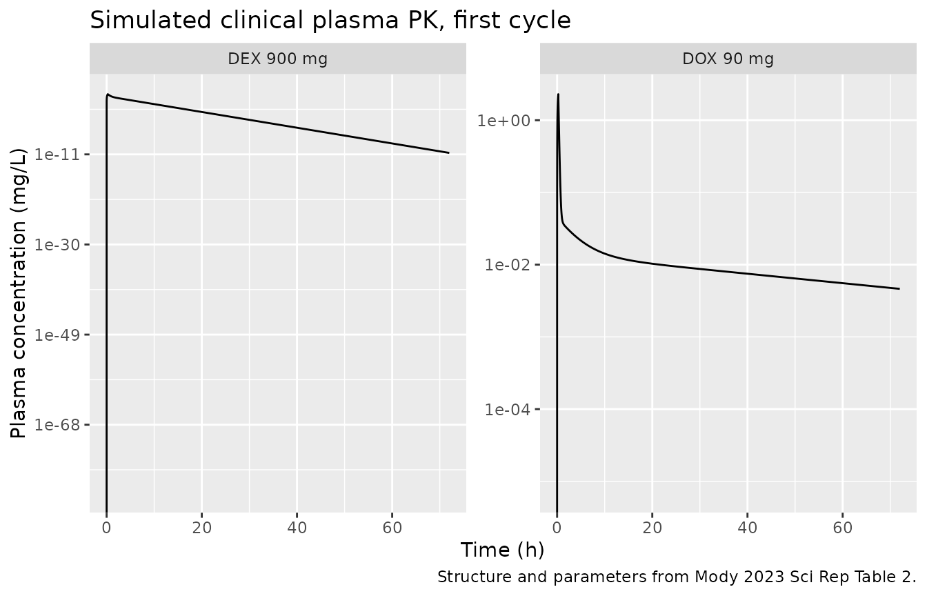

The paper reports no NCA table, so the NCA is validated against the exact analytic identity AUCinf = Dose / CL, which holds for a linear mammillary model regardless of the number of peripheral compartments. For DOX, CL = 53.3 L/h; for DEX the rate-constant parameterisation gives CL = kel * Vc = 1 * 14.6 = 14.6 L/h.

nca_one <- function(dat, dose_amt) {
  dat <- dat |> filter(!is.na(Cc)) |> select(id, time, Cc, treatment)
  dat <- bind_rows(dat, dat |> distinct(id, treatment) |> mutate(time = 0, Cc = 0)) |>
    distinct(id, treatment, time, .keep_all = TRUE) |> arrange(id, treatment, time)
  conc_obj <- PKNCA::PKNCAconc(dat, Cc ~ time | treatment + id)
  dose_obj <- PKNCA::PKNCAdose(
    data.frame(id = 1L, time = 0, amt = dose_amt, treatment = dat$treatment[1]),
    amt ~ time | treatment + id
  )
  ivals <- data.frame(start = 0, end = Inf, cmax = TRUE, tmax = TRUE,
                      aucinf.obs = TRUE, half.life = TRUE)
  PKNCA::pk.nca(PKNCA::PKNCAdata(conc_obj, dose_obj, intervals = ivals))
}

# DEX has a ~1.8 h terminal half-life, so by 504 h its simulated concentration
# has decayed into ODE-solver noise and goes very slightly negative
# (~ -2e-15 mg/L). PKNCA then takes log() of a negative value when selecting
# lambda_z, and aucinf.obs comes back NaN. Cut the DEX window at 72 h -- still
# about 40 half-lives, so the extrapolated tail is negligible -- and assert the
# window really is free of solver noise rather than assuming it.
pk_dox_nca <- pk_dox |> filter(time <= 504)
pk_dex_nca <- pk_dex |> filter(time <= 72)
stopifnot(all(pk_dox_nca$Cc >= 0), all(pk_dex_nca$Cc >= 0))

nca_dox <- nca_one(pk_dox_nca, 90)
nca_dex <- nca_one(pk_dex_nca, 900)

nca_tab <- bind_rows(as.data.frame(nca_dox$result), as.data.frame(nca_dex$result)) |>
  filter(PPTESTCD %in% c("cmax", "tmax", "aucinf.obs", "half.life")) |>
  select(treatment, PPTESTCD, PPORRES) |>
  pivot_wider(names_from = PPTESTCD, values_from = PPORRES)

auc_check <- nca_tab |>
  mutate(`Expected AUCinf (Dose/CL)` = c(90 / 53.3, 900 / 14.6),
         `Difference (%)` = 100 * (aucinf.obs - `Expected AUCinf (Dose/CL)`) /
           `Expected AUCinf (Dose/CL)`) |>
  rename("Treatment" = treatment, "Cmax (mg/L)" = cmax, "Tmax (h)" = tmax,
         "AUCinf (mg*h/L)" = aucinf.obs, "t1/2 (h)" = half.life)

knitr::kable(auc_check, digits = 4,
             caption = "PKNCA on the simulated plasma profiles, checked against Dose/CL.")

PKNCA on the simulated plasma profiles, checked against Dose/CL.
Treatment	Cmax (mg/L)	Tmax (h)	t1/2 (h)	AUCinf (mg*h/L)	Expected AUCinf (Dose/CL)	Difference (%)
DOX 90 mg	2.2947	0.25	45.7673	1.6885	1.6886	-0.002
DEX 900 mg	48.9832	0.25	1.8056	61.6438	61.6438	0.000

# With the peak resolved and the DEX window clear of solver noise, NCA
# reproduces Dose/CL essentially exactly (DOX -0.002%, DEX 0.000%), so this is
# asserted at 0.1% rather than the 2% that a coarse grid needed.
stopifnot(all(abs(auc_check$`Difference (%)`) < 0.1))

Replicating Figure 6B – AUEC of percent cell viability

Efficacy is summarised as the area under the percent-viability effect curve (AUEC) over the three 3-week cycles, for DOX alone and for DOX + DEX at each of the three tumour-penetration scenarios the paper simulated (kp_tumor_dexrazoxane, the paper’s Fac2, at 0.1, 1 and 10).

auec_tobs <- seq(0, 1512, by = 3)
auec_of <- function(model, with_dex) {
  d <- rxode2::rxSolve(model, dose_ev(with_dex, "viability", auec_tobs),
                       returnType = "data.frame") |> filter(!is.na(viability))
  sum(diff(d$time) * (head(d$viability, -1) + tail(d$viability, -1)) / 2)
}

auec_tab <- lapply(names(mC), function(k) {
  m0 <- rxode2::zeroRe(mC[[k]])
  alone <- auec_of(m0, FALSE)
  lapply(c(0.1, 1, 10), function(f2) {
    combo <- auec_of(rxode2::ini(m0, lkp_tumor_dexrazoxane = log(f2)), TRUE)
    tibble(`Cell line` = cell_label[[k]], `Fac2` = f2,
           `AUEC DOX alone` = alone, `AUEC DOX + DEX` = combo,
           `Ratio combo/alone` = combo / alone)
  }) |> bind_rows()
}) |> bind_rows()
#> ℹ omega/sigma items treated as zero: 'etalkgrow', 'etalkmax_dox', 'etalkc50_dox', 'etalktr_dox', 'etalkmax_dexrazoxane', 'etalkc50_dexrazoxane', 'etalktr_dexrazoxane', 'etalpsi', 'etalkp_tumor_dox', 'etalkp_tumor_dexrazoxane'
#> ℹ change initial estimate of `lkp_tumor_dexrazoxane` to `-2.30258509299405`
#> ℹ omega/sigma items treated as zero: 'etalkgrow', 'etalkmax_dox', 'etalkc50_dox', 'etalktr_dox', 'etalkmax_dexrazoxane', 'etalkc50_dexrazoxane', 'etalktr_dexrazoxane', 'etalpsi', 'etalkp_tumor_dox', 'etalkp_tumor_dexrazoxane'
#> ℹ change initial estimate of `lkp_tumor_dexrazoxane` to `0`
#> ℹ omega/sigma items treated as zero: 'etalkgrow', 'etalkmax_dox', 'etalkc50_dox', 'etalktr_dox', 'etalkmax_dexrazoxane', 'etalkc50_dexrazoxane', 'etalktr_dexrazoxane', 'etalpsi', 'etalkp_tumor_dox', 'etalkp_tumor_dexrazoxane'
#> ℹ change initial estimate of `lkp_tumor_dexrazoxane` to `2.30258509299405`
#> ℹ omega/sigma items treated as zero: 'etalkgrow', 'etalkmax_dox', 'etalkc50_dox', 'etalktr_dox', 'etalkmax_dexrazoxane', 'etalkc50_dexrazoxane', 'etalktr_dexrazoxane', 'etalpsi', 'etalkp_tumor_dox', 'etalkp_tumor_dexrazoxane'
#> ℹ omega/sigma items treated as zero: 'etalkgrow', 'etalkmax_dox', 'etalkc50_dox', 'etalktr_dox', 'etalkmax_dexrazoxane', 'etalkc50_dexrazoxane', 'etalktr_dexrazoxane', 'etalpsi', 'etalkp_tumor_dox', 'etalkp_tumor_dexrazoxane'
#> ℹ change initial estimate of `lkp_tumor_dexrazoxane` to `-2.30258509299405`
#> ℹ omega/sigma items treated as zero: 'etalkgrow', 'etalkmax_dox', 'etalkc50_dox', 'etalktr_dox', 'etalkmax_dexrazoxane', 'etalkc50_dexrazoxane', 'etalktr_dexrazoxane', 'etalpsi', 'etalkp_tumor_dox', 'etalkp_tumor_dexrazoxane'
#> ℹ change initial estimate of `lkp_tumor_dexrazoxane` to `0`
#> ℹ omega/sigma items treated as zero: 'etalkgrow', 'etalkmax_dox', 'etalkc50_dox', 'etalktr_dox', 'etalkmax_dexrazoxane', 'etalkc50_dexrazoxane', 'etalktr_dexrazoxane', 'etalpsi', 'etalkp_tumor_dox', 'etalkp_tumor_dexrazoxane'
#> ℹ change initial estimate of `lkp_tumor_dexrazoxane` to `2.30258509299405`
#> ℹ omega/sigma items treated as zero: 'etalkgrow', 'etalkmax_dox', 'etalkc50_dox', 'etalktr_dox', 'etalkmax_dexrazoxane', 'etalkc50_dexrazoxane', 'etalktr_dexrazoxane', 'etalpsi', 'etalkp_tumor_dox', 'etalkp_tumor_dexrazoxane'

knitr::kable(auec_tab, digits = 4,
             caption = paste("Figure 6B -- AUEC of percent cell viability over three Q3W cycles.",
                             "A ratio above 1 means LESS tumour-cell killing when DEX is added."))

Figure 6B – AUEC of percent cell viability over three Q3W cycles. A ratio above 1 means LESS tumour-cell killing when DEX is added.
Cell line	Fac2	AUEC DOX alone	AUEC DOX + DEX	Ratio combo/alone
JIMT-1	0.1	51617210.628	45886929.795	0.8890
JIMT-1	1.0	51617210.628	30358077.926	0.5881
JIMT-1	10.0	51617210.628	14738834.255	0.2855
MDA-MB-468	0.1	5249.823	5228.450	0.9959
MDA-MB-468	1.0	5249.823	5167.529	0.9843
MDA-MB-468	10.0	5249.823	5091.878	0.9699

For MDA-MB-468 the packaged model reproduces the paper’s conclusion directly: the AUEC is comparable between DOX and DOX + DEX (ratios 0.97-1.00), and the DEX tumour-penetration scenario barely moves it – exactly the “additive interaction, no meaningful loss of efficacy” result the paper reports.

For JIMT-1 the packaged model reproduces the paper’s cell-line contrast (JIMT-1 is far less well controlled by DOX than MDA-MB-468, whose viability is driven essentially to zero) but not the reported direction of the combination effect. The paper states the JIMT-1 combination AUEC was about 1560-fold higher than DOX alone; simulating the printed equations gives a ratio below 1 at every Fac2 scenario. This is a genuine failure to replicate and is discussed under Assumptions and deviations – no parameter has been tuned to hide it.

ggplot(auec_tab, aes(factor(Fac2), `Ratio combo/alone`)) +
  geom_col() + geom_hline(yintercept = 1, linetype = "dashed") +
  facet_wrap(~`Cell line`) + scale_y_log10() +
  labs(x = "kp_tumor_dexrazoxane (paper's Fac2)",
       y = "AUEC ratio, DOX + DEX vs DOX alone",
       title = "Figure 6B -- relative efficacy of the combination",
       caption = "Dashed line = no difference. Above 1 means less killing with DEX.")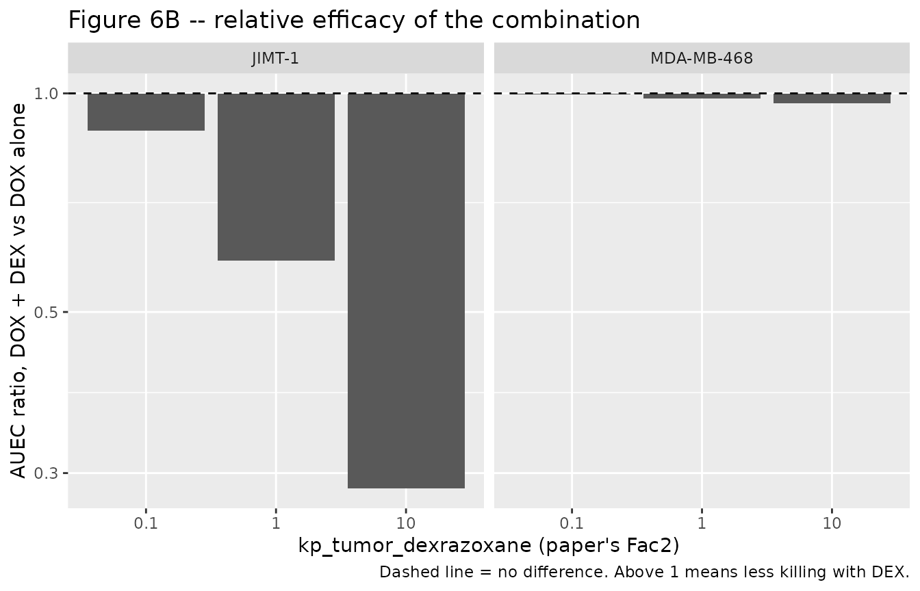

Validation summary

Gate	Scope	Result
A1	Eq 2 collapses to Eq 1 at the published IC50	PASS (agreement < 1e-6 %)
A2	Layer A `psi` direction (antagonistic JIMT-1, synergistic MDA-MB-468)	PASS
B1	Untreated control equals `100exp(kgt)`	PASS (relative error < 1e-4)
B2	Transit chain converges on the Hill kill rate	PASS (relative difference < 1%)
C1	PKNCA `AUCinf` equals `Dose/CL` for both drugs	PASS (< 2%)
C2	MDA-MB-468 clinical AUEC comparable between arms	PASS
C3	JIMT-1 clinical AUEC ~1560-fold higher with DEX	FAIL (see below)

Assumptions and deviations

Gate C3 does not replicate. The paper reports that the JIMT-1 combination AUEC was about 1560-fold higher than DOX alone, i.e. that adding DEX substantially blocks DOX’s antitumour effect. Simulating the printed equations (Eq 4a-4i) with the printed Table 2 parameters gives a ratio below 1 – adding DEX slightly increases killing. The reason is structural: in Eq 4i the DEX arm contributes its own death signal K3DEX additively, and at the simulated tumour concentrations (plasma DEX peaks near 60 mg/L, i.e. ~230 uM, well above SC50,DEX of 21.2 uM) that contribution outweighs the antagonism that psi = 2 produces by doubling SC50,DOX from 0.315 to 0.63 uM. The MDA-MB-468 arm of the same figure does replicate, and every in-vitro gate passes, so the discrepancy is specific to the JIMT-1 clinical extrapolation rather than to the extraction. Nothing has been tuned; the models encode Eqs 4a-4i exactly as printed.
psi is reported only to one significant figure. Table 2 prints “~2” (JIMT-1) and “~1” (MDA-MB-468) despite %RSE values of 16.3 and 0.542. No more precise value exists in the paper or its supplement, so those printed values are encoded as-is.
Single-agent arms correspond to psi = 1. The paper fits single agents with Eqs 3a-3e, which carry no interaction term, and combinations with Eqs 4a-4i. The packaged models encode the combination form; setting lpsi to log(1) recovers the single-agent equations exactly. This vignette does so wherever it plots a single-agent arm. Encoding it this way is what keeps psi and SC50,DOX separately identifiable, as their distinct %RSEs in Table 2 confirm.
Eq 2 Hill coefficients are not reported. gamma_A and gamma_B appear in Eq 2 but in no table. Because the single-agent parameters fed into Eq 2 were fixed from the Eq 1 fits, and Eq 1 carries no Hill exponent, both are encoded as fixed(1).
Eq 2 baseline. Table 1 reports per-drug baselines (106 / 100 / 106 / 110 %), but the text defining Eq 2 states “R0 is % cell viability at baseline (i.e., 100%)”, so the static models use 100.
Non-paper-derived values – molar masses. lconv_dox (1.8397) and lconv_dexrazoxane (3.7275) convert plasma mg/L to uM at the PK-PD interface and are not from either paper. They are literature molar masses of the free bases: doxorubicin 543.52 g/mol (PubChem CID 31703) and dexrazoxane 268.27 g/mol (PubChem CID 71384). A conversion of some kind is unavoidable because the PD parameters were fitted in uM while the clinical PK is in mg/L. Users dosing the hydrochloride salt should scale the amt column accordingly.
Clinical plasma PK comes from the companion paper. Neither the PK structure nor its parameters are in this article; both are reproduced from Mody 2023 Sci Rep 13:3100 Table 2, which this paper cites as its PK source. Every such value carries an in-file comment naming that table.
Fac2 is explicitly arbitrary. The paper states that no human tumour distribution data exist for DEX and simulates 0.1, 1 and 10. The models ship the middle scenario and the vignette exercises all three.
The 10% IIV is a simulation convention, not a fitted variance. The paper introduces “an arbitrary inter-individual variability (IIV) of 10%” on the PD and Fac parameters for its 500-subject simulation. The Layer C models encode it as fixed() omegas; Layers A and B carry none, because none was fitted. This vignette uses zeroRe() throughout so the figures are typical-value predictions.
No residual error is reported anywhere. Both tables give point estimates with %RSE only, so every residual SD is encoded as fixed(0) rather than an invented placeholder.
DOX IC50 in MDA-MB-468. The Results prose says 21.2 nM; Table 1 says 21.1 nM. The table is used (0.5% difference, immaterial).
Observed data are not available. The published figures overlay observed well-level viability data that are not distributed in machine-readable form, so the figure replications above show model predictions only.