CKD-519, CETP activity, HDL-C and LDL-C (Kim 2020)
Source:vignettes/articles/Kim_2020_CKD_519.Rmd
Kim_2020_CKD_519.RmdModel and source
- Citation: Kim CO, Jeon S, Han S, Park MS, Yim DS. A Population Pharmacokinetic and Pharmacodynamic Model of CKD-519. Pharmaceutics. 2020;12(6):573. doi:10.3390/pharmaceutics12060573. PK: Table 2 and Equations 1-3; CETP activity: Table 3 and Equations 4-6; HDL-C and LDL-C: Table 4 and Equations 7-10; model structure: Figure 1.
- Description: Sequential population PK/PD model for the cholesteryl ester transfer protein (CETP) inhibitor CKD-519 in healthy adult men given 50-400 mg once daily with a standard meal for 14 days (Kim 2020). PK: three-compartment disposition with an Erlang absorption chain (dose into four transit compartments at Ktr, then an absorption compartment draining to central at Ka) and a relative bioavailability that falls with dose (Bmax * (1 - DOSE / (BA50 + DOSE))) and, for the 50-200 mg cohorts only, decays exponentially with time since the first dose. CETP activity is a turnover state whose first-order loss is stimulated by an Emax function of plasma CKD-519 and whose production rises with time on study (placebo Emax-in-time effect). HDL-C and LDL-C are turnover states whose first-order elimination is respectively stimulated (HDL-C) and inhibited (LDL-C) by a sigmoid function of CETP activity; LDL-C production also rises linearly with time (placebo).
- Article: https://doi.org/10.3390/pharmaceutics12060573 (open access; PMC7356970)
CKD-519 is an oral inhibitor of cholesteryl ester transfer protein (CETP) that was developed for dyslipidaemia. Its exposure is highly variable: it depends on food, it rises less than dose-proportionally, and in the 50-200 mg cohorts it falls on repeated dosing. Kim et al. fitted a sequential population PK/PD model to a two-week multiple-ascending-dose study in healthy men. The chain has three links:
-
PK. Three-compartment disposition. Absorption runs
through five sequential compartments: four transit compartments at
Ktr, then an absorption compartment that drains to central atKa. The relative bioavailability falls with dose and, below 400 mg, decays with time since the first dose. - CETP activity. A turnover model. Plasma CKD-519 stimulates the first-order loss of CETP activity through an Emax function. CETP production rises with time on study, a placebo effect that is also seen in the placebo group.
- HDL-C and LDL-C. Turnover models driven by CETP activity through a sigmoid Emax function. CETP activity stimulates HDL-C elimination and inhibits LDL-C elimination, so inhibiting CETP raises HDL-C and lowers LDL-C. LDL-C production also rises linearly with time (placebo effect).
The paper fitted the three stages one after another, each using the
individual parameters of the previous stage. The packaged model joins
them into one ODE system with four outputs: Cc (ng/mL),
cetp (pmol), hdl and ldl
(mg/dL).
Population
Thirty-two healthy Korean men took part: six on CKD-519 and two on placebo in each of four cohorts (50, 100, 200 and 400 mg). Their mean age was 32.2 years (19-47) and their mean weight 68.7 kg (58.3-79.5) (Table 1). CKD-519 or placebo was given once daily with a standard breakfast (700-800 kcal, 5-25% fat) for 14 days. Subjects stayed in hospital from day 1 to day 21. The data were 1392 plasma CKD-519 concentrations, 2064 CETP activity values and 656 HDL-C and LDL-C values. Age, weight, BMI, MDRD creatinine clearance and ALT were screened as covariates, and none was retained in any final model.
The same information is available programmatically via
readModelDb("Kim_2020_CKD_519")()$population.
Source trace
Every ini() value carries an in-file comment in
inst/modeldb/specificDrugs/Kim_2020_CKD_519.R. The table
collects them.
| Equation / parameter | Value | Source location |
|---|---|---|
Absorption chain: 5 sequential compartments, 4 at Ktr
then 1 at Ka
|
n/a | Figure 1; Section 3.2 |
| 3-compartment disposition | n/a | Figure 1; Table 2 |
F = BA * FT |
n/a | Equation 1 |
BA = Bmax * (1 - DOSE / (BA50 + DOSE)) |
n/a | Equation 2; Table 2 |
FT = exp(-alpha * TIME) |
n/a | Equation 3; Table 2 |
lcl (CL/F) |
6.4 L/h | Table 2 |
lvc (V/F) |
11.4 L | Table 2 |
lvp (V2/F) |
45.4 L | Table 2 |
lvp2 (V3/F) |
1006 L | Table 2 |
lq (Q2/F) |
2.6 L/h | Table 2 |
lq2 (Q3/F) |
3.3 L/h | Table 2 |
lka (Ka) |
1.09 1/h | Table 2 |
lktr (Ktr) |
1.10 1/h | Table 2 |
lfdepot_max (Bmax) |
1.6 | Table 2 |
ld50_fdepot (BA50) |
90.1 mg | Table 2 |
alpha_fdepot (alpha1, 50-200 mg) |
0.002 1/h | Table 2 |
alpha_fdepot_high (alpha2, 400 mg) |
0 (fixed) | Table 2; Section 3.2 |
etalcl, etalvp2,
etalfdepot_max, etalktr
|
15.6, 58.1, 28.2, 14.1 %CV | Table 2 |
propSd / addSd (CKD-519) |
0.30 / 0.0001 (fixed) | Table 2 |
dCETP/dt = Kin,base (1 + Placebo) - Kout (1 + Drug) CETP |
n/a | Equation 4; Figure 1 |
Placebo = Kmax T / (K50 + T) |
n/a | Equation 5; Table 3 |
Drug = Emax Cp / (EC50 + Cp) |
n/a | Equation 6; Table 3 |
lrbase_cetp (CETPbase) |
350 pmol | Table 3 |
lkin_cetp (Kin,base) |
164 pmol/h | Table 3 |
lpbo_emax_cetp (Kmax) |
9.6 | Table 3 |
lpbo_t50_cetp (K50) |
9700 h | Table 3 |
lemax (Emax) |
18.2 | Table 3 |
lec50 (EC50) |
587 ng/mL | Table 3 |
etalkin_cetp, etalemax
|
19.7, 39.5 %CV | Table 3 |
addSd_cetp / propSd_cetp
|
40.4 pmol / 0.112 | Table 3 |
dHDL/dt = Ksyn - Kdeg HDL (1 + RES) |
n/a | Equation 7 |
dLDL/dt = Ksyn (1 + PLA) - Kdeg LDL (1 - RES) |
n/a | Equation 8; Table 4; Figure 1 |
RES = CETP^gamma Rmax / (CETP^gamma + R50^gamma) |
n/a | Equation 9; Table 4 |
PLA = beta * time |
n/a | Equation 10; Table 4 |
lrbase_hdl (RB) |
50.0 mg/dL | Table 4, HDL-C |
lksyn_hdl (Ksyn) |
1.26 mg/dL/h | Table 4, HDL-C |
lhill_hdl (gamma) |
2.1 | Table 4, HDL-C |
lemax_hdl (Rmax) |
1.5 | Table 4, HDL-C |
lec50_hdl (R50) |
185 pmol | Table 4, HDL-C |
etalrbase_hdl |
17.2 %CV | Table 4, HDL-C |
addSd_hdl / propSd_hdl
|
4.6 mg/dL / 0.0001 (fixed) | Table 4, HDL-C |
lrbase_ldl (RB) |
97.4 mg/dL | Table 4, LDL-C |
lksyn_ldl (Ksyn) |
0.435 mg/dL/h | Table 4, LDL-C |
lpbo_slope_ldl (beta) |
0.0009 1/h | Table 4, LDL-C |
lhill_ldl (gamma) |
2.2 | Table 4, LDL-C |
lemax_ldl (Rmax) |
0.8 | Table 4, LDL-C |
lec50_ldl (R50) |
80.7 pmol | Table 4, LDL-C |
etalrbase_ldl, etalpbo_slope_ldl,
etalhill_ldl
|
23.6, 97.4, 50.9 %CV | Table 4, LDL-C |
propSd_ldl |
0.07 (additive 0 fixed, omitted) | Table 4, LDL-C |
kout_cetp, kdeg_hdl,
kdeg_ldl
|
derived | Pre-dose steady state (see Assumptions) |
The IIV rows are reported as CV%. They are converted to log-normal
variances with omega^2 = log(CV^2 + 1).
Virtual cohort
The study had five arms: 50, 100, 200 and 400 mg once daily for 14
days, and placebo. Each arm below has 40 virtual subjects. The model has
no demographic covariates, so each subject needs only the dose
(DOSE) and the 400 mg indicator (DOSE_HIGH).
Observations run hourly to day 21 (504 h). They sit on the
cetp state, which is one of the declared endpoints, and
rxode2 returns Cc, hdl and ldl at
the same rows.
arms <- tibble::tribble(
  ~arm,      ~dose,
  "Placebo",     0,
  "50 mg",      50,
  "100 mg",    100,
  "200 mg",    200,
  "400 mg",    400
) |>
  mutate(arm = factor(arm, levels = arm))

n_per_arm <- 40L
dose_times <- seq(0, 13 * 24, by = 24)
obs_times <- sort(unique(c(seq(0, 504, by = 1), 312 + c(0.25, 0.5, 0.75))))

make_arm <- function(arm, dose, ids) {
  subj <- tibble(id = ids, arm = arm, dose_mg = dose, DOSE = dose, DOSE_HIGH = as.integer(dose == 400))
  obs <- tidyr::crossing(subj, time = obs_times) |>
    mutate(evid = 0L, amt = NA_real_, cmt = "cetp")
  if (dose == 0) {
    return(obs)
  }
  doses <- tidyr::crossing(subj, time = dose_times) |>
    mutate(evid = 1L, amt = dose, cmt = "transit1")
  bind_rows(doses, obs)
}

events <- bind_rows(lapply(seq_len(nrow(arms)), function(i) {
  make_arm(
    as.character(arms$arm[i]), arms$dose[i],
    ids = (i - 1L) * n_per_arm + seq_len(n_per_arm)
  )
})) |>
  arrange(id, time, desc(evid)) |>
  # rxode2 reads a column named DOSE as the dose amount unless the standard
  # event columns come first, so put them first.
  select(id, time, evid, amt, cmt, everything())

stopifnot(!anyDuplicated(unique(events[, c("id", "time", "evid")])))
Simulation
mod <- readModelDb("Kim_2020_CKD_519")

rxode2::rxSetSeed(519)
sim <- rxode2::rxSolve(
  mod,
  events = events,
  keep = c("arm", "dose_mg"),
  useLinCmt = FALSE
) |>
  as.data.frame() |>
  mutate(arm = factor(arm, levels = levels(arms$arm)))
#> ℹ parameter labels from comments will be replaced by 'label()'

# Typical-value solve (no IIV, no residual error). The paper's Figure 4 is a
# typical-value simulation. `omega = NA, sigma = NA` is used instead of
# zeroRe(), which is not safe on multi-endpoint models.
events_typ <- events |>
  group_by(arm) |>
  filter(id == min(id)) |>
  ungroup()
sim_typ <- rxode2::rxSolve(
  mod,
  events = events_typ,
  keep = c("arm", "dose_mg"),
  omega = NA,
  sigma = NA,
  useLinCmt = FALSE
) |>
  as.data.frame() |>
  mutate(arm = factor(arm, levels = levels(arms$arm)))
Replicate published figures
Figure 3: visual predictive checks
# Replicates the layout of Figure 3 of Kim 2020 (VPC of CKD-519, CETP
# activity, HDL-C and LDL-C). `Cc`, `cetp`, `hdl` and `ldl` are the individual
# predictions without residual error.
vpc <- sim |>
  select(arm, time, Cc, cetp, hdl, ldl) |>
  tidyr::pivot_longer(c(Cc, cetp, hdl, ldl), names_to = "output") |>
  group_by(arm, output, time) |>
  summarise(
    q05 = quantile(value, 0.05),
    q50 = median(value),
    q95 = quantile(value, 0.95),
    .groups = "drop"
  ) |>
  mutate(output = factor(
    output,
    levels = c("Cc", "cetp", "hdl", "ldl"),
    labels = c("CKD-519 (ng/mL)", "CETP activity (pmol)", "HDL-C (mg/dL)", "LDL-C (mg/dL)")
  ))

ggplot(vpc, aes(time / 24, q50, colour = arm, fill = arm)) +
  geom_ribbon(aes(ymin = q05, ymax = q95), alpha = 0.12, colour = NA) +
  geom_line() +
  facet_wrap(~output, scales = "free_y", ncol = 1) +
  labs(
    x = "Time since first dose (days)", y = NULL, colour = NULL, fill = NULL,
    caption = "Median and 5th-95th percentiles of 40 simulated subjects per arm."
  ) +
  theme_bw()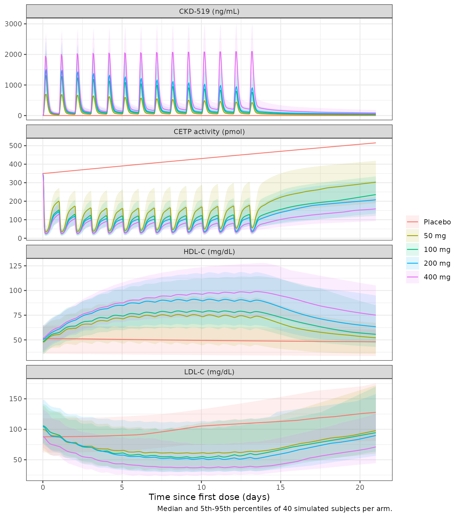
Figure 4: HDL-C and LDL-C change from baseline
The paper simulated the typical HDL-C and LDL-C response to 21 days of daily dosing and marked a target of a 40% change from baseline. It reports that the responses peak after about ten days of dosing, that they then decline slowly at 50-200 mg but not at 400 mg, and that the 40% targets are reached at 200 and 400 mg.
# Replicates Figure 4 of Kim 2020 (typical-value simulation, 21 days of
# once-daily dosing, IIV and residual error excluded as in Section 2.5).
events_fig4 <- bind_rows(lapply(seq_len(nrow(arms))[-1], function(i) {
  d <- arms$dose[i]
  subj <- tibble(id = i, arm = as.character(arms$arm[i]), DOSE = d, DOSE_HIGH = as.integer(d == 400))
  bind_rows(
    tidyr::crossing(subj, time = seq(0, 20 * 24, by = 24)) |>
      mutate(evid = 1L, amt = d, cmt = "transit1"),
    tidyr::crossing(subj, time = seq(0, 21 * 24, by = 2)) |>
      mutate(evid = 0L, amt = NA_real_, cmt = "cetp")
  )
})) |>
  arrange(id, time, desc(evid)) |>
  select(id, time, evid, amt, cmt, everything())

fig4 <- rxode2::rxSolve(
  mod,
  events = events_fig4,
  keep = c("arm"),
  omega = NA,
  sigma = NA,
  useLinCmt = FALSE
) |>
  as.data.frame() |>
  mutate(arm = factor(arm, levels = levels(arms$arm))) |>
  group_by(arm) |>
  mutate(
    `HDL-C` = 100 * (hdl / first(hdl) - 1),
    `LDL-C` = 100 * (ldl / first(ldl) - 1)
  ) |>
  ungroup()

fig4 |>
  select(arm, time, `HDL-C`, `LDL-C`) |>
  tidyr::pivot_longer(c(`HDL-C`, `LDL-C`), names_to = "lipid", values_to = "pct") |>
  ggplot(aes(time / 24, pct, colour = arm)) +
  geom_line() +
  geom_hline(
    data = data.frame(lipid = c("HDL-C", "LDL-C"), target = c(40, -40)),
    aes(yintercept = target), linetype = "dashed"
  ) +
  facet_wrap(~lipid, scales = "free_y") +
  labs(
    x = "Time since first dose (days)", y = "Change from baseline (%)",
    colour = NULL, caption = "Dashed lines: the paper's 40% targets."
  ) +
  theme_bw()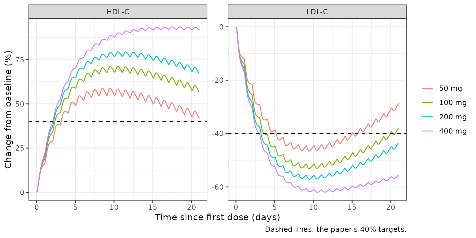
fig4_summary <- fig4 |>
  group_by(arm) |>
  summarise(
    hdl_peak_pct = max(`HDL-C`),
    hdl_peak_day = time[which.max(`HDL-C`)] / 24,
    hdl_day21_pct = `HDL-C`[time == 504],
    ldl_nadir_pct = min(`LDL-C`),
    ldl_nadir_day = time[which.min(`LDL-C`)] / 24,
    ldl_day21_pct = `LDL-C`[time == 504],
    .groups = "drop"
  )

fig4_summary |>
  dplyr::rename(
    "Arm" = arm,
    "HDL-C peak (%)" = hdl_peak_pct,
    "HDL-C peak day" = hdl_peak_day,
    "HDL-C day 21 (%)" = hdl_day21_pct,
    "LDL-C nadir (%)" = ldl_nadir_pct,
    "LDL-C nadir day" = ldl_nadir_day,
    "LDL-C day 21 (%)" = ldl_day21_pct
  ) |>
knitr::kable(digits = 1, caption = "Typical-value lipid response to 21 days of dosing.")| Arm | HDL-C peak (%) | HDL-C peak day | HDL-C day 21 (%) | LDL-C nadir (%) | LDL-C nadir day | LDL-C day 21 (%) |
|---|---|---|---|---|---|---|
| 50 mg | 58.8 | 9.5 | 41.6 | -46.6 | 9.4 | -28.6 |
| 100 mg | 71.2 | 10.5 | 56.4 | -53.2 | 9.5 | -37.8 |
| 200 mg | 79.5 | 11.5 | 67.1 | -57.2 | 9.5 | -43.5 |
| 400 mg | 93.5 | 17.5 | 91.8 | -62.0 | 10.5 | -55.6 |
The maintainers digitised the Figure 4 curves at their peak (HDL-C) and nadir (LDL-C). The HDL-C panel is reproduced. The Discussion also states the maximal responses: HDL-C rises to 160-190% of baseline and LDL-C falls by 47-66%.
fig4_digitised <- tibble::tribble(
  ~arm,     ~hdl_peak_fig4, ~ldl_nadir_fig4,
  "50 mg",              80,              72,
  "100 mg",             86,              64,
  "200 mg",             90,              58,
  "400 mg",             97,              51
)

fig4_cmp <- fig4_summary |>
  mutate(arm = as.character(arm)) |>
  inner_join(fig4_digitised, by = "arm") |>
  mutate(
    hdl_peak_sim = 50 * (1 + hdl_peak_pct / 100),
    ldl_nadir_sim = 97.4 * (1 + ldl_nadir_pct / 100),
    hdl_pct_diff = 100 * (hdl_peak_sim / hdl_peak_fig4 - 1),
    ldl_pct_diff = 100 * (ldl_nadir_sim / ldl_nadir_fig4 - 1)
  )

fig4_cmp |>
  select(arm, hdl_peak_sim, hdl_peak_fig4, hdl_pct_diff, ldl_nadir_sim, ldl_nadir_fig4, ldl_pct_diff) |>
  dplyr::rename(
    "Arm" = arm,
    "HDL-C peak, model (mg/dL)" = hdl_peak_sim,
    "HDL-C peak, Figure 4 (mg/dL)" = hdl_peak_fig4,
    "HDL-C difference (%)" = hdl_pct_diff,
    "LDL-C nadir, model (mg/dL)" = ldl_nadir_sim,
    "LDL-C nadir, Figure 4 (mg/dL)" = ldl_nadir_fig4,
    "LDL-C difference (%)" = ldl_pct_diff
  ) |>
knitr::kable(digits = 1, caption = "Typical-value peaks and nadirs against Figure 4 (digitised).")| Arm | HDL-C peak, model (mg/dL) | HDL-C peak, Figure 4 (mg/dL) | HDL-C difference (%) | LDL-C nadir, model (mg/dL) | LDL-C nadir, Figure 4 (mg/dL) | LDL-C difference (%) |
|---|---|---|---|---|---|---|
| 50 mg | 79.4 | 80 | -0.7 | 52.0 | 72 | -27.8 |
| 100 mg | 85.6 | 86 | -0.5 | 45.6 | 64 | -28.7 |
| 200 mg | 89.7 | 90 | -0.3 | 41.7 | 58 | -28.1 |
| 400 mg | 96.7 | 97 | -0.3 | 37.0 | 51 | -27.5 |
stopifnot(
  # HDL-C peak reproduces Figure 4 (digitised to about +/-2 mg/dL); realised
  # differences are within 1-5%.
  all(abs(fig4_cmp$hdl_pct_diff) < 10),
  # Discussion: maximal HDL-C increase 160-190% of baseline (realised 159-194%).
  all(fig4_cmp$hdl_peak_sim / 50 > 1.50 & fig4_cmp$hdl_peak_sim / 50 < 2.05),
  # Discussion: maximal LDL-C decrease 47-66% (realised 47-62%).
  all(-fig4_cmp$ldl_nadir_pct > 40 & -fig4_cmp$ldl_nadir_pct < 70),
  # Section 3.5: 40% HDL-C increase and 40% LDL-C decrease reached at 200 and 400 mg.
  all(fig4_summary$hdl_peak_pct[fig4_summary$arm %in% c("200 mg", "400 mg")] > 40),
  all(fig4_summary$ldl_nadir_pct[fig4_summary$arm %in% c("200 mg", "400 mg")] < -40),
  # Section 3.5: responses peak after about ten days of dosing at 50-200 mg and
  # then decline, while the 400 mg response is sustained to day 21.
  all(fig4_summary$hdl_peak_day[fig4_summary$arm %in% c("50 mg", "100 mg", "200 mg")] > 6),
  all(fig4_summary$hdl_peak_day[fig4_summary$arm %in% c("50 mg", "100 mg", "200 mg")] < 15),
  with(fig4_summary[fig4_summary$arm == "400 mg", ], hdl_peak_pct - hdl_day21_pct < 2)
)
The LDL-C panel of Figure 4 is not reproduced: its
curves sit about 38% above the model’s in every arm, from the nadir to
day 20, while starting at the same baseline. The discrepancy is in the
source, not the implementation. Figure 4’s LDL-C curves (a 26-47%
maximal decrease) contradict the paper’s own Discussion (47-66%), which
the model matches. They also contradict the observed LDL-C medians in
the Figure 3 VPC (next section), which the model also matches. The HDL-C
panel of Figure 4 is driven by the same CETP trajectory and is
reproduced. The maintainers tested two alternative readings, and neither
recovers the LDL-C panel. Applying the time term
(1 + beta T) twice (Table 4 and Equation 8 read literally
together) raises the late curve but not the nadir. Replacing the final
estimates with the bootstrap medians changes the curves by less than 3
mg/dL.
Figure 3: observed medians
The Figure 3 VPC plots the observed data. The maintainers read the median line of each panel at three landmarks: the HDL-C peak, the LDL-C nadir, and CETP activity at 480 h, a week after the last dose. The typical-value solve of the 14-day study design is compared against them.
fig3_digitised <- tibble::tribble(
  ~arm,     ~hdl_peak, ~ldl_nadir, ~cetp_480,
  "50 mg",         80,         55,       270,
  "100 mg",        82,         55,       230,
  "200 mg",        92,         42,       190,
  "400 mg",        95,         42,       150
)

fig3_sim <- sim_typ |>
  filter(dose_mg > 0) |>
  group_by(arm) |>
  summarise(
    hdl_peak = max(hdl),
    ldl_nadir = min(ldl),
    cetp_480 = cetp[time == 480],
    .groups = "drop"
  ) |>
  mutate(arm = as.character(arm))

fig3_cmp <- fig3_sim |>
  tidyr::pivot_longer(-arm, names_to = "landmark", values_to = "model") |>
  inner_join(
    fig3_digitised |> tidyr::pivot_longer(-arm, names_to = "landmark", values_to = "figure_3"),
    by = c("arm", "landmark")
  ) |>
  mutate(pct_diff = 100 * (model / figure_3 - 1))

fig3_cmp |>
  dplyr::rename(
    "Arm" = arm, "Landmark" = landmark, "Model" = model,
    "Figure 3 median" = figure_3, "Difference (%)" = pct_diff
  ) |>
knitr::kable(digits = 1, caption = "Typical-value landmarks against the observed medians of Figure 3 (digitised).")| Arm | Landmark | Model | Figure 3 median | Difference (%) |
|---|---|---|---|---|
| 50 mg | hdl_peak | 79.4 | 80 | -0.7 |
| 50 mg | ldl_nadir | 52.0 | 55 | -5.5 |
| 50 mg | cetp_480 | 264.8 | 270 | -1.9 |
| 100 mg | hdl_peak | 85.6 | 82 | 4.4 |
| 100 mg | ldl_nadir | 45.6 | 55 | -17.1 |
| 100 mg | cetp_480 | 218.8 | 230 | -4.9 |
| 200 mg | hdl_peak | 89.7 | 92 | -2.5 |
| 200 mg | ldl_nadir | 41.7 | 42 | -0.7 |
| 200 mg | cetp_480 | 188.6 | 190 | -0.7 |
| 400 mg | hdl_peak | 96.3 | 95 | 1.4 |
| 400 mg | ldl_nadir | 37.0 | 42 | -11.9 |
| 400 mg | cetp_480 | 139.7 | 150 | -6.9 |
PKNCA validation
The paper reports no NCA table for this study. Its Discussion quotes the observed apparent clearance by dose group (11.98 L/h at 50 mg, 30.04 L/h at 200 mg and 23.98 L/h at 400 mg) and a terminal half-life of 145.4-166.2 h. It also states that at 400 mg the AUC after repeated dosing was three times the AUC after the first dose. The NCA below computes the day-1 and day-14 dosing intervals and the terminal half-life after the last dose.
sim_nca <- sim |>
  filter(!is.na(Cc), dose_mg > 0) |>
  select(id, time, Cc, arm) |>
  mutate(arm = droplevels(arm))

dose_df <- events |>
  filter(evid == 1) |>
  select(id, time, amt, arm) |>
  mutate(arm = factor(arm, levels = levels(sim_nca$arm)))

conc_obj <- PKNCA::PKNCAconc(sim_nca, Cc ~ time | arm + id)
dose_obj <- PKNCA::PKNCAdose(dose_df, amt ~ time | arm + id)

intervals <- data.frame(
  start = c(0, 312, 312),
  end = c(24, 336, 504),
  cmax = c(TRUE, TRUE, FALSE),
  tmax = c(TRUE, TRUE, FALSE),
  auclast = c(TRUE, TRUE, FALSE),
  cl.last = c(FALSE, TRUE, FALSE),
  half.life = c(FALSE, FALSE, TRUE)
)

nca_res <- PKNCA::pk.nca(PKNCA::PKNCAdata(conc_obj, dose_obj, intervals = intervals))

nca_tab <- as.data.frame(nca_res) |>
  filter(PPTESTCD %in% c("cmax", "tmax", "auclast", "cl.last", "half.life")) |>
  mutate(period = case_when(
    start == 0 ~ "day 1",
    end == 336 ~ "day 14",
    TRUE ~ "after last dose"
  )) |>
  # cl.last is Dose / AUC in mg / (ng*h/mL); x 1000 gives L/h.
  mutate(PPORRES = ifelse(PPTESTCD == "cl.last", 1000 * PPORRES, PPORRES)) |>
  group_by(arm, period, PPTESTCD) |>
  summarise(median = median(PPORRES, na.rm = TRUE), .groups = "drop")

nca_tab |>
  mutate(parameter = paste(PPTESTCD, period, sep = ", ")) |>
  select(arm, parameter, median) |>
  tidyr::pivot_wider(names_from = parameter, values_from = median) |>
  dplyr::rename("Arm" = arm) |>
knitr::kable(digits = 1, caption = "Median simulated NCA parameters (Cc in ng/mL, time in h, AUC in ng*h/mL, CL in L/h).")| Arm | half.life, after last dose | tmax, after last dose | auclast, day 1 | cmax, day 1 | tmax, day 1 | auclast, day 14 | cl.last, day 14 | cmax, day 14 | tmax, day 14 |
|---|---|---|---|---|---|---|---|---|---|
| 50 mg | 331.3 | 5 | 4420.0 | 729.4 | 5 | 3510.5 | 14.2 | 438.4 | 5 |
| 100 mg | 371.1 | 5 | 7903.7 | 1323.0 | 5 | 5750.7 | 17.4 | 775.3 | 5 |
| 200 mg | 332.1 | 5 | 9299.1 | 1515.7 | 5 | 7328.6 | 27.3 | 918.3 | 5 |
| 400 mg | 288.5 | 5 | 11466.8 | 1992.3 | 5 | 15989.6 | 25.0 | 2143.6 | 5 |
Comparison against published values
day14 <- as.data.frame(nca_res) |>
  filter(start == 312, end == 336, PPTESTCD == "cl.last")
hl <- as.data.frame(nca_res) |>
  filter(start == 312, end == 504, PPTESTCD == "half.life")

# PKNCA's cl.last uses the day-14 AUC over the dosing interval, so it is the
# steady-state apparent clearance Dose / AUCtau (reported in L/h after the
# unit conversion below: mg / (ng*h/mL) = 1000 L/h).
day14 <- day14 |> mutate(PPORRES = PPORRES * 1000)

published <- tibble::tribble(
  ~arm,     ~cl.last,
  "50 mg",     11.98,
  "200 mg",    30.04,
  "400 mg",    23.98
)

cmp <- nlmixr2lib::ncaComparisonTable(
  simulated = day14 |> filter(arm %in% published$arm),
  reference = published,
  by = "arm",
  units = c(cl.last = "L/h"),
  tolerance_pct = 20
)
#> Warning: ncaParamLabel(): unknown PKNCA code(s) returned as-is: 'cl.last'
knitr::kable(cmp, caption = "Day-14 apparent clearance, simulated vs. Kim 2020 Discussion. * differs by >20%.")| NCA parameter | arm | Reference | Simulated | % diff |
|---|---|---|---|---|
| cl.last (L/h) | 50 mg | 12 | 14.2 | +18.9% |
| cl.last (L/h) | 200 mg | 30 | 27.3 | -9.1% |
| cl.last (L/h) | 400 mg | 24 | 25 | +4.3% |
# Typical-value day-1 AUC0-24 and day-14 AUCtau by the trapezoidal rule on the
# hourly grid, and the steady-state CL/F = Dose / AUCtau (L/h).
auc_typ <- function(time, conc, from) {
  i <- time >= from & time <= from + 24
  sum(diff(time[i]) * (head(conc[i], -1) + tail(conc[i], -1)) / 2)
}
typ <- sim_typ |>
  filter(dose_mg > 0) |>
  group_by(arm) |>
  summarise(
    dose = first(dose_mg),
    auc_d1 = auc_typ(time, Cc, 0),
    auc_d14 = auc_typ(time, Cc, 312),
    .groups = "drop"
  ) |>
  mutate(
    arm = as.character(arm),
    cl_ss = 1000 * dose / auc_d14,
    ratio = auc_d14 / auc_d1
  )

cl_typ <- typ |>
  inner_join(published, by = "arm") |>
  mutate(pct_diff = 100 * (cl_ss / cl.last - 1))

typ |>
  select(arm, cl_ss, ratio) |>
  dplyr::rename(
    "Arm" = arm,
    "Day-14 CL/F, typical (L/h)" = cl_ss,
    "AUC ratio, day 14 / day 1" = ratio
  ) |>
knitr::kable(digits = 2, caption = "Typical-value steady-state CL/F and accumulation ratio.")| Arm | Day-14 CL/F, typical (L/h) | AUC ratio, day 14 / day 1 |
|---|---|---|
| 50 mg | 12.99 | 0.79 |
| 100 mg | 17.62 | 0.79 |
| 200 mg | 26.89 | 0.79 |
| 400 mg | 26.28 | 1.37 |
stopifnot(
  # Day-14 CL/F by dose group (typical value, deterministic); realised
  # -10% to +10%. A mis-transcribed CL/F, Bmax, BA50 or alpha1 moves it by far
  # more.
  all(abs(cl_typ$pct_diff) < 25),
  # Section 3.2: exposure falls on repeated dosing at 50-200 mg (realised
  # ratio 0.79) but not at 400 mg (realised 1.37).
  all(typ$ratio[typ$arm != "400 mg"] < 0.9),
  typ$ratio[typ$arm == "400 mg"] > 1.2
)

hl |>
  group_by(arm) |>
  summarise(half_life_h = median(PPORRES, na.rm = TRUE)) |>
  dplyr::rename("Arm" = arm, "Median terminal half-life (h)" = half_life_h) |>
knitr::kable(digits = 0, caption = "Terminal half-life after the last dose (Discussion: 145.4-166.2 h).")| Arm | Median terminal half-life (h) |
|---|---|
| 50 mg | 331 |
| 100 mg | 371 |
| 200 mg | 332 |
| 400 mg | 288 |
Day-14 apparent clearance reproduces the Discussion values. Three exposure figures do not, and the maintainers did not find a reading of the model that explains them:
- Accumulation at 400 mg. Section 3.2 states that the 400 mg AUC after repeated dosing was three times the first-dose AUC. The final model gives a typical ratio of about 1.4. It does reproduce the direction: exposure falls on repeated dosing at 50-200 mg and rises at 400 mg.
-
Half-life. The simulated terminal half-life after
the last dose is about 290-370 h, twice the observed 145.4-166.2 h, over
a similar 192 h window. It is set by the slow third compartment
(
V3/F = 1006 L,Q3/F = 3.3 L/h). The paper does not say how its half-life was estimated. -
Tmax. The Discussion describes absorption as
delayed, with a Tmax of about 1 h. Five sequential compartments at
Ktr = 1.10andKa = 1.09 1/hgive a mean absorption time of about 4.6 h, and the simulated Tmax is 5 h.
Assumptions and deviations
-
Kout, Kdeg(HDL-C) and Kdeg(LDL-C) are derived. The
paper does not tabulate the first-order loss constants. They are set so
that each turnover state starts at steady state at its tabulated
baseline:
Kout = Kin,base / CETPbase,Kdeg,HDL = Ksyn / (RB (1 + RES0))andKdeg,LDL = Ksyn / (RB (1 - RES0)), whereRES0is the CETP-activity effect (Equation 9) at the baseline CETP activity of 350 pmol. The effect is not zero at baseline, so it has to enter the steady-state balance. -
The CETP loss term includes the state. Printed
Equation 4 writes the loss as
Kout x (1 + Drug)without the CETP activity. The text definesKoutas a first-order rate constant and Figure 1 draws it as a loss from the CETP state, so the loss isKout x (1 + Drug) x CETP. -
The LDL-C time effect enters once. Table 4 writes
Ksy = Ksyn x (1 + beta T)and Equation 8 writesKsy x (1 + PLA)withPLA = beta x time. Read literally together, the time term would enter twice. Figure 1 labels the LDL-C inputKsyn,base x (1 + beta x T), so the model applies(1 + beta t)once to the tabulatedKsyn. - Ksyn units. Table 4 prints the unit of both Ksyn values as ‘h-1’. Both enter Equations 7 and 8 as zero-order production rates, so the model treats them as mg/dL/h.
- HDL-C proportional error. Table 4 prints the HDL-C proportional residual error as ‘0.0.0001 FIX’. It is read as 0.0001 fixed, the same placeholder as the fixed CKD-519 additive error in Table 2. The LDL-C additive error is 0 fixed and is omitted.
- Residual error as standard deviations. The sigma rows are read as standard deviations. The paper does not state whether they are variances or SDs. The values (30% proportional for CKD-519, 40.4 pmol additive for CETP activity against a baseline of 350 pmol) are plausible as SDs.
-
Time.
TIMEin Equation 3 andTin the placebo terms are time since the first dose, so the simulation starts dosing att = 0. The 400 mg indicatorDOSE_HIGHswitchesalphato its fixed value of 0, as in Table 2. The paper defines the switch by dose group, so the model is not defined for doses between 200 and 400 mg. -
Placebo subjects receive no dose. Their
DOSEvalue does not matter because bioavailability never acts; 0 is used. - No correction notice for this article was found on the journal page as of 2026-09-26.