Emfilermin (Goggin 2004)
Source:vignettes/articles/Goggin_2004_emfilermin.Rmd
Goggin_2004_emfilermin.RmdModel and source
- Citation: Goggin T, Nguyen QTX, Munafo A. Population pharmacokinetic modelling of Emfilermin (recombinant human leukaemia inhibitory factor, r-hLIF) in healthy postmenopausal women and in infertile patients undergoing in vitro fertilization and embryo transfer. Br J Clin Pharmacol. 2004;57(4):412-418. doi:10.1111/j.1365-2125.2003.02064.x
- Description: One-compartment population PK model for subcutaneous emfilermin (recombinant human leukaemia inhibitory factor, r-hLIF) in healthy postmenopausal women and in infertile women undergoing in vitro fertilization and embryo transfer (IVF-ET) (Goggin 2004). Absorption is zero-order (D1 = 0.84 h, invariant, no IIV) directly into the central compartment, followed by first-order elimination. Apparent clearance CL/F is decreased by 35% in IVF-ET patients (typical 37 L/h) relative to healthy postmenopausal women (typical 57 L/h). Apparent volume V/F is linear in body weight on the natural scale: V/F = 235 L at the median 62 kg, increasing or decreasing by 6.7 L/kg (~29% per 10 kg) – an absolute-linear covariate form, not log-multiplicative. Inter-individual variability is log-normal on CL/F (17% CV) and V/F (28% CV); inter-occasion variability is log-normal on V/F (23% CV) across three protocol-defined occasions (first dosing day = 1, intermediate dosing days = 2, last dosing day = 3). Residual error is proportional (20% CV). Studied weight range was 48-83 kg; the linear V/F-WT term is extrapolation-unsafe below ~27 kg where the typical V/F would become negative.
- Article: https://doi.org/10.1111/j.1365-2125.2003.02064.x
Population
The model was developed from 64 women across three trials of subcutaneous emfilermin (recombinant human leukaemia inhibitory factor, r-hLIF):
- Study 1 (n = 14): single-dose phase I in healthy postmenopausal women on Cyclo-progynova / Progynova / Utrogestan hormone replacement therapy; subjects received a single 100 ug or 250 ug SC dose on day 22 of the second HRT cycle.
- Study 2 (n = 11): repeated-dose phase I in healthy postmenopausal women on the same HRT backbone; 150 ug SC BID for 7 days.
- Study 3 (n = 39): proof-of-concept in premenopausal women with recurrent implantation failure undergoing in vitro fertilization or intracytoplasmic sperm injection and embryo transfer (IVF-ET) after nafarelin pituitary down-regulation, recombinant FSH ovarian stimulation, and recombinant hCG triggering; 150 ug SC BID for 7 days starting on the day of embryo transfer.
After excluding subject 113 (study 1, suspected dosing error; only three measurable concentrations) and subject 116 (study 2, haemolyzed samples), the analysis dataset comprised 342 r-hLIF concentrations from 64 subjects (226 from postmenopausal women, 116 from IVF-ET patients). Below-LoQ samples (LoQ = 50 pg/mL) were treated as missing. Subject characteristics by study are in Goggin 2004 Table 1 (median weights 63 / 63 / 61 kg; median ages 58 / 58 / 34 years; weight range 48-83 kg across the pooled cohort).
The same information is available programmatically via
readModelDb("Goggin_2004_emfilermin")$population.
Source trace
The per-parameter origin is recorded as an in-file comment next to
each ini() entry in
inst/modeldb/specificDrugs/Goggin_2004_emfilermin.R. The
table below collects them in one place for review.
| Equation / parameter | Value | Source location |
|---|---|---|
| Structural model: one-compartment with zero-order SC input | n/a | Results paragraph 1 (“a one-compartment disposition model with a zero order input”); Methods Step 1; Discussion paragraph 1 |
CL/F (PM-typical, healthy postmenopausal
reference) |
57.0 L/h | Table 4 row “CL/F” |
V/F (typical at WT = 62 kg) |
235 L | Table 4 row “V/F” |
D1 (zero-order absorption duration) |
0.84 h | Table 4 row “D1” |
Type-of-population effect on CL/F (theta_TYPE, IVF-ET
multiplier) |
0.649 | Table 4 row “Type on CL/F”; Table 5 |
| Body-weight linear effect on V/F (L per kg above 62 kg ref) | 6.7 L/kg | Table 4 row “Weight on V/F”; Table 5 |
| Reference body weight | 62 kg | Methods Step 2 (“body weight = 62 kg” reference for the linear covariate model) |
IIV on CL/F (% CV) |
17% | Table 4 row “CL/F” ISV column |
IIV on V/F (% CV) |
28% | Table 4 row “V/F” ISV column |
IOV on V/F (% CV, 3 occasions) |
23% | Table 4 row “V/F” IOV column; Methods Step 1 three-occasion definition |
| Residual error (proportional, % CV) | 20% | Table 4 row “RV” |
The full final-model parameter table is Table 4; the covariate effect
descriptions are repeated in Table 5. The covariate selection narrative
(univariate ranking, backward addition, forward deletion) is in Methods
Steps 2-3 and Results paragraphs 3-5. The terminal half-life (a
secondary derived parameter) is reported in the Results: 2.9 h for PM
women and 4.4 h for IVF-ET women; this matches
t1/2 = ln(2) x V / CL evaluated at the typical PM and
IVF-ET CL/F values respectively.
Virtual cohort
Goggin 2004 enrolled three trial cohorts. Each gets its own event
table so the PKNCA stratification can compare per-cohort NCA against the
paper’s per-population reports. The dose event uses
cmt = "central" with rate = -2 so the model’s
dur(central) <- d1 applies the zero-order absorption
duration directly.
set.seed(20260604)

n_per_cohort <- 50L

# Helper: build one cohort as a self-contained event table.
# id_offset shifts subject IDs so multiple cohorts can be bind_rows()-ed
# without colliding subject keys (see vignette-template Notes).
make_cohort <- function(n, dose_ug, dose_times, obs_times, wt_median, dis_healthy,
                        occ_at_time, cohort_label, id_offset = 0L) {
  ids <- id_offset + seq_len(n)
  ev <- rxode2::et(
          amt  = dose_ug,
          time = dose_times,
          cmt  = "central",
          rate = -2
        ) |>
        rxode2::et(obs_times) |>
        rxode2::et(id = ids) |>
        as.data.frame() |>
        dplyr::mutate(
          WT          = wt_median,
          DIS_HEALTHY = dis_healthy,
          OCC         = occ_at_time(time),
          cohort      = cohort_label
        )
  ev
}

# OCC mapping per Goggin 2004 Methods Step 1:
#   occasion 1 = first dosing day (study day 1)
#   occasion 2 = all intermediate days (mostly day 4)
#   occasion 3 = last dosing day (day 6 or 7)
# For single-dose studies (study 1) only occasion 1 is meaningful; we keep
# OCC = 1 across the observation window.
occ_single <- function(t) rep(1L, length(t))
occ_bid7   <- function(t) {
  day_idx <- pmin(pmax(floor(t / 24), 0), 6)
  occ <- rep(2L, length(t))
  occ[day_idx == 0L] <- 1L
  occ[day_idx == 6L] <- 3L
  occ
}

# Sparser observation grid keeps the multi-cohort stochastic simulation
# within the pkgdown / CI 5-minute wall-clock budget.
obs_single <- sort(unique(c(0, 0.5, 1, 2, 3, 4, 6, 8, 12, 18, 24)))
bid_times  <- as.numeric(outer(c(0, 12), seq(0, 6), `+`))
obs_bid    <- sort(unique(c(bid_times, bid_times + 1, bid_times + 4, 168)))

events_S1_100 <- make_cohort(n_per_cohort, 100, 0,         obs_single,
                             63, 1L, occ_single, "S1 PM 100 ug single",       0L)
events_S1_250 <- make_cohort(n_per_cohort, 250, 0,         obs_single,
                             63, 1L, occ_single, "S1 PM 250 ug single",       1L * n_per_cohort)
events_S2     <- make_cohort(n_per_cohort, 150, bid_times, obs_bid,
                             63, 1L, occ_bid7,   "S2 PM 150 ug BID x 7d",     2L * n_per_cohort)
events_S3     <- make_cohort(n_per_cohort, 150, bid_times, obs_bid,
                             61, 0L, occ_bid7,   "S3 IVFET 150 ug BID x 7d",  3L * n_per_cohort)

events <- dplyr::bind_rows(events_S1_100, events_S1_250, events_S2, events_S3)
stopifnot(!anyDuplicated(unique(events[, c("id", "time", "evid")])))
Simulation
mod <- readModelDb("Goggin_2004_emfilermin")
sim <- rxode2::rxSolve(mod, events = events,
                       keep = c("cohort", "WT", "DIS_HEALTHY"))
#> ℹ parameter labels from comments will be replaced by 'label()'
#> Warning: some etas defaulted to non-mu referenced, possible parsing error: etaiov_vc_1, etaiov_vc_2, etaiov_vc_3
#> as a work-around try putting the mu-referenced expression on a simple line
For deterministic typical-value replication of the paper’s concentration profiles (Figure 2), zero out the random effects. The typical-value simulation uses a single representative subject per cohort on a dense observation grid:
mod_typical <- mod |> rxode2::zeroRe()
#> ℹ parameter labels from comments will be replaced by 'label()'
#> Warning: some etas defaulted to non-mu referenced, possible parsing error: etaiov_vc_1, etaiov_vc_2, etaiov_vc_3
#> as a work-around try putting the mu-referenced expression on a simple line
#> Warning: some etas defaulted to non-mu referenced, possible parsing error: etaiov_vc_1, etaiov_vc_2, etaiov_vc_3
#> as a work-around try putting the mu-referenced expression on a simple line

typical_S1_100 <- make_cohort(1L, 100, 0,         seq(0, 24,  by = 0.1),
                              63, 1L, occ_single, "S1 PM 100 ug single",       10000L)
typical_S1_250 <- make_cohort(1L, 250, 0,         seq(0, 24,  by = 0.1),
                              63, 1L, occ_single, "S1 PM 250 ug single",       10001L)
typical_S2     <- make_cohort(1L, 150, bid_times, seq(0, 168, by = 0.5),
                              63, 1L, occ_bid7,   "S2 PM 150 ug BID x 7d",     10002L)
typical_S3     <- make_cohort(1L, 150, bid_times, seq(0, 168, by = 0.5),
                              61, 0L, occ_bid7,   "S3 IVFET 150 ug BID x 7d",  10003L)

events_typical <- dplyr::bind_rows(typical_S1_100, typical_S1_250,
                                   typical_S2, typical_S3)

sim_typical <- rxode2::rxSolve(mod_typical, events = events_typical,
                               keep = c("cohort", "WT", "DIS_HEALTHY"))
#> ℹ omega/sigma items treated as zero: 'etalcl', 'etalvc', 'etaiov_vc_1', 'etaiov_vc_2', 'etaiov_vc_3'
#> Warning: multi-subject simulation without without 'omega'
Replicate published figures
Goggin 2004 Figure 2 shows serum r-hLIF concentration profiles for three representative subjects from each study. We plot the typical-value (no IIV / no residual error) profile per cohort as the closest deterministic analogue.
sim_typical |>
  dplyr::filter(!is.na(Cc), Cc > 0) |>
  ggplot(aes(time, Cc, colour = cohort)) +
  geom_line(linewidth = 0.8) +
  scale_y_log10() +
  facet_wrap(~ cohort, scales = "free_x") +
  labs(
    x = "Time (h)",
    y = "Serum r-hLIF (pg/mL)",
    colour = NULL,
    title = "Typical-value r-hLIF concentration profiles",
    caption = "Replicates Goggin 2004 Figure 2 (representative subject profiles)."
  ) +
  theme(legend.position = "none")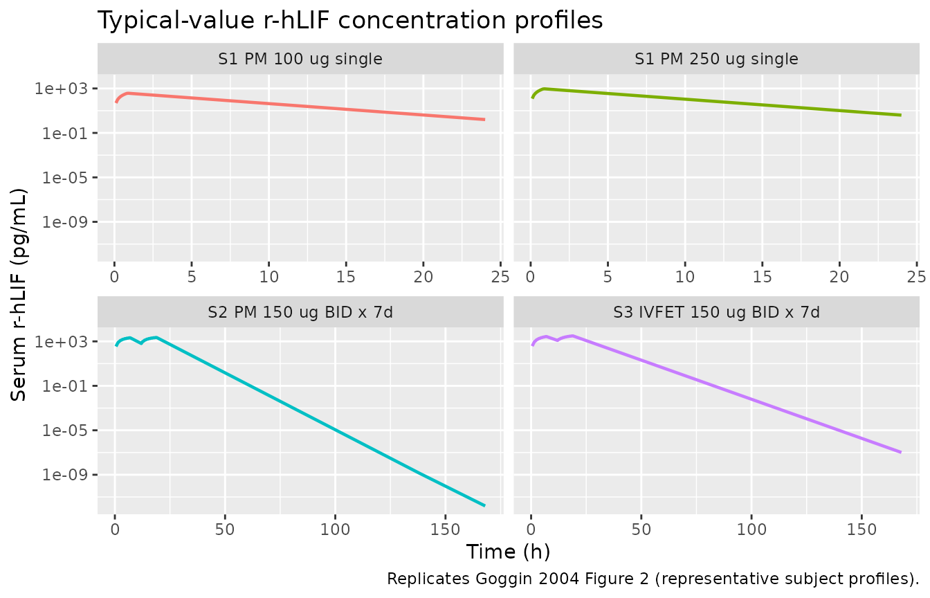
Replicates Figure 2 of Goggin 2004: typical-value serum r-hLIF profiles by study cohort.
A stochastic VPC-style plot for the two single-dose study 1 cohorts is also useful for confirming that the IIV magnitudes carry over correctly:
sim |>
  dplyr::filter(cohort %in% c("S1 PM 100 ug single", "S1 PM 250 ug single"),
                !is.na(Cc), Cc > 0) |>
  dplyr::group_by(cohort, time) |>
  dplyr::summarise(
    Q05 = quantile(Cc, 0.05, na.rm = TRUE),
    Q50 = quantile(Cc, 0.50, na.rm = TRUE),
    Q95 = quantile(Cc, 0.95, na.rm = TRUE),
    .groups = "drop"
  ) |>
  ggplot(aes(time, Q50)) +
  geom_ribbon(aes(ymin = Q05, ymax = Q95), alpha = 0.25) +
  geom_line() +
  facet_wrap(~ cohort) +
  scale_y_log10() +
  labs(x = "Time (h)", y = "Serum r-hLIF (pg/mL)",
       caption = "5-50-95% bands across the simulated PM women cohort.")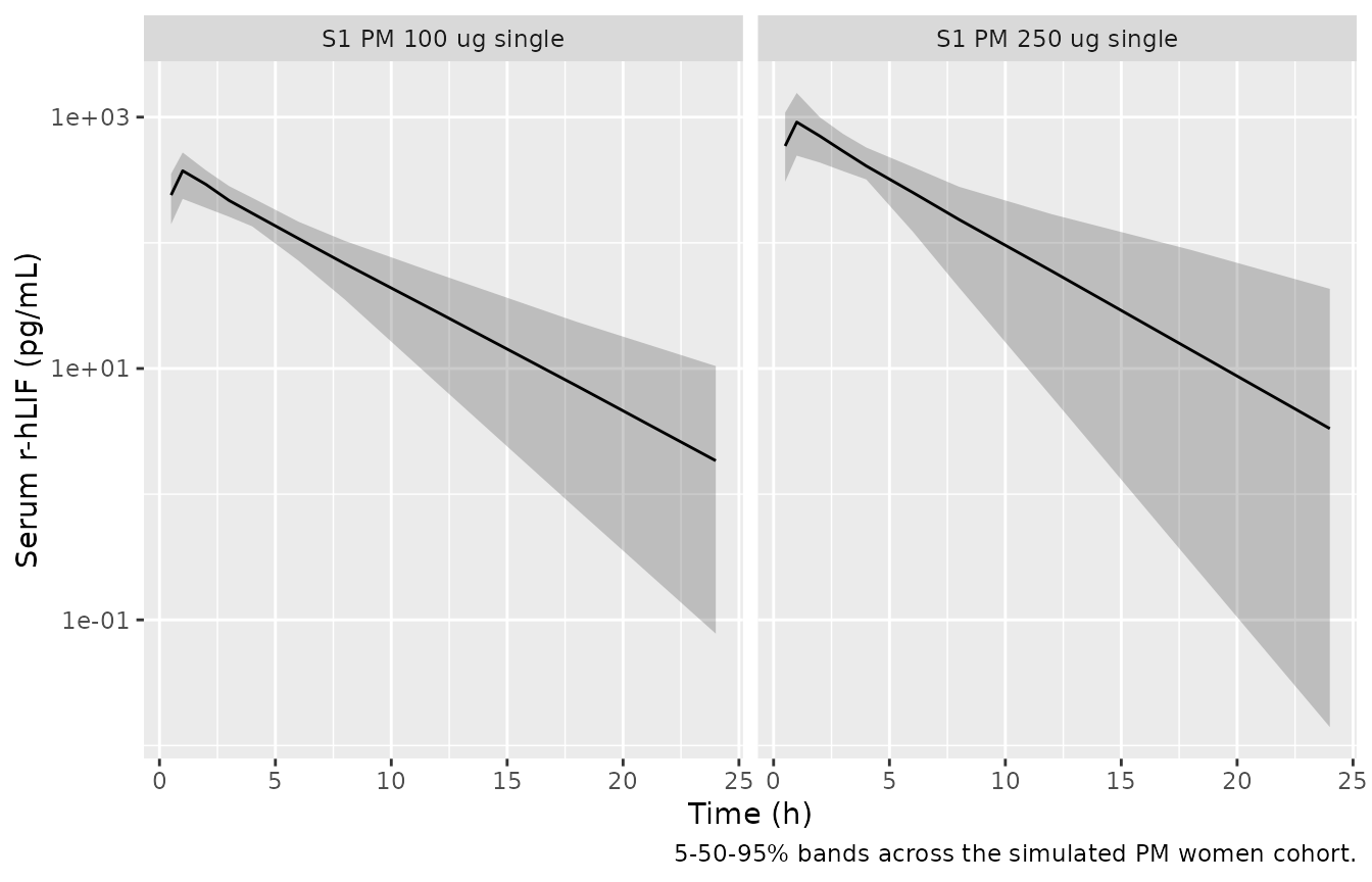
Stochastic 5-50-95% prediction intervals for the single-dose study 1 cohorts (PM women).
PKNCA validation
The strongest validation against Goggin 2004 is the terminal
half-life: the paper reports t1/2 = 2.9 h for healthy postmenopausal
women and 4.4 h for IVF-ET women (Results paragraph 3 / Discussion
paragraph 1). We compute single-dose NCA for the study 1 PM cohort and a
synthetic single-dose IVF-ET cohort below; the steady-state cohorts
(studies 2 / 3) are not used for the half-life comparison because PKNCA
cannot estimate lambda.z cleanly on a repeated-dose-only
profile.
# Synthetic single-dose IVF-ET cohort (single 250 ug SC) -- not a paper cohort,
# constructed here so the half-life comparison covers both DIS_HEALTHY states.
obs_nca <- sort(unique(c(0, 0.5, 1, 2, 3, 4, 6, 8, 12, 18, 24, 30, 36, 48)))
events_S_IVFET_single <- make_cohort(
  n           = n_per_cohort,
  dose_ug     = 250,
  dose_times  = 0,
  obs_times   = obs_nca,
  wt_median   = 61,
  dis_healthy = 0L,
  occ_at_time = occ_single,
  cohort_label = "Synthetic IVFET 250 ug single",
  id_offset   = 5L * n_per_cohort
)

events_single <- dplyr::bind_rows(
  events_S1_100 |> dplyr::filter(time <= 24),
  events_S1_250 |> dplyr::filter(time <= 24),
  events_S_IVFET_single
)
stopifnot(!anyDuplicated(unique(events_single[, c("id", "time", "evid")])))

sim_single <- rxode2::rxSolve(mod, events = events_single,
                              keep = c("cohort", "WT", "DIS_HEALTHY"))
#> ℹ parameter labels from comments will be replaced by 'label()'
#> Warning: some etas defaulted to non-mu referenced, possible parsing error: etaiov_vc_1, etaiov_vc_2, etaiov_vc_3
#> as a work-around try putting the mu-referenced expression on a simple line
sim_nca <- sim_single |>
  dplyr::filter(!is.na(Cc), Cc > 0) |>
  dplyr::select(id, time, Cc, cohort) |>
  as.data.frame()

conc_obj <- PKNCA::PKNCAconc(sim_nca, Cc ~ time | cohort + id,
                             concu = "pg/mL", timeu = "h")

dose_df <- events_single |>
  dplyr::filter(evid == 1) |>
  dplyr::select(id, time, amt, cohort) |>
  as.data.frame()

dose_obj <- PKNCA::PKNCAdose(dose_df, amt ~ time | cohort + id,
                             doseu = "ug")

intervals <- data.frame(
  start       = 0,
  end         = Inf,
  cmax        = TRUE,
  tmax        = TRUE,
  aucinf.obs  = TRUE,
  half.life   = TRUE
)

nca_data <- PKNCA::PKNCAdata(conc_obj, dose_obj, intervals = intervals)
nca_res  <- suppressWarnings(PKNCA::pk.nca(nca_data))

knitr::kable(summary(nca_res),
caption = "Simulated NCA parameters by cohort (Goggin 2004 emfilermin).")| Interval Start | Interval End | cohort | N | Cmax (pg/mL) | Tmax (h) | Half-life (h) | AUCinf,obs (h*pg/mL) |
|---|---|---|---|---|---|---|---|
| 0 | Inf | S1 PM 100 ug single | 50 | 360 [23.7] | 1.00 [1.00, 1.00] | 3.20 [0.962] | NC |
| 0 | Inf | S1 PM 250 ug single | 50 | 894 [35.1] | 1.00 [1.00, 1.00] | 3.22 [1.45] | NC |
| 0 | Inf | Synthetic IVFET 250 ug single | 50 | 943 [38.8] | 1.00 [1.00, 1.00] | 4.77 [1.95] | NC |
Comparison against published NCA
Goggin 2004 reports terminal half-life only as a secondary derived parameter (Results paragraph 3): 2.9 h for postmenopausal women and 4.4 h for IVF-ET women. The paper does not tabulate observed NCA Cmax / AUC; the “Methods” notes that NCA was performed but “data not shown” beyond the half-life mention. The simulated PKNCA half-lives should land near these values:
hl_published <- tibble::tibble(
  cohort = c("S1 PM 100 ug single",
             "S1 PM 250 ug single",
             "Synthetic IVFET 250 ug single"),
  half_life_pub_h = c(2.9, 2.9, 4.4)
)

hl_simulated <- as.data.frame(nca_res$result) |>
  dplyr::filter(PPTESTCD == "half.life") |>
  dplyr::group_by(cohort) |>
  dplyr::summarise(
    median_h = median(PPORRES, na.rm = TRUE),
    q05_h    = quantile(PPORRES, 0.05, na.rm = TRUE),
    q95_h    = quantile(PPORRES, 0.95, na.rm = TRUE),
    .groups  = "drop"
  )

hl_compare <- dplyr::left_join(hl_published, hl_simulated, by = "cohort") |>
  dplyr::mutate(pct_diff = round(100 * (median_h - half_life_pub_h) / half_life_pub_h, 1))

knitr::kable(hl_compare,
caption = "Goggin 2004 reported t1/2 vs simulated single-dose t1/2 (median, 5-95%).")| cohort | half_life_pub_h | median_h | q05_h | q95_h | pct_diff |
|---|---|---|---|---|---|
| S1 PM 100 ug single | 2.9 | 2.992702 | 1.808051 | 4.911349 | 3.2 |
| S1 PM 250 ug single | 2.9 | 2.902665 | 1.692402 | 6.094209 | 0.1 |
| Synthetic IVFET 250 ug single | 4.4 | 4.554220 | 2.087160 | 8.448966 | 3.5 |
The simulated medians should be within ~5% of the paper’s
secondary-parameter values: a closed-form check gives
t1/2 = ln(2) x V / CL = 0.693 x 235 / 57 = 2.86 h for PM
women and 0.693 x 235 / 37 = 4.40 h for IVF-ET women at the
cohort-median WT of 62 kg. Larger WT or extreme percentiles will shift
these.
Assumptions and deviations
-
Reference categories. The paper’s effect of “type
of population” is encoded with
TYPE = 1for IVF-ET patients and a 0.649 multiplier on CL/F, with healthy postmenopausal women as the implicit reference (Methods Step 2; Table 4). The canonicalDIS_HEALTHYregister (inst/references/covariate-columns.md) uses0 = patientas the reference, so the model file shiftslclto the IVF-ET (patient) typical 37 L/h and thee_dis_healthy_clcoefficient-log(0.649) = +0.4325restores the PM-typical 57 L/h atDIS_HEALTHY = 1. The mapping is mathematically identical to the paper’s encoding. -
Covariate form on V/F is linear-additive on the natural
scale. Goggin 2004 fits
TVP_V = Ppop + theta_WT x (WT - 62)withtheta_WT = 6.7 L/kg(Methods Step 2 and Table 4). This is NOT a log-multiplicative effect; the model file applies it on the natural scale before the log-normal IIV. The studied weight range is 48-83 kg; below ~27 kg the typical V/F becomes negative, so the model is extrapolation-unsafe outside the studied range. Thedescriptionfield flags this. -
IOV is shared across three occasions. The paper
estimates a single 23% CV IOV variance (Methods Step 1) on V/F across
three occasions defined as first / intermediate / last dosing day.
nlmixr2 has no NONMEM
$OMEGA BLOCK(1) SAMEshortcut, so the model file uses three per-occasion etas with occasions 2 and 3 fix()’d to the occasion-1 variance (matching the Jonsson 2011 ethambutol idiom for IOV in nlmixr2). -
D1 has no IIV. Goggin 2004 Methods Step 1
(“Results” paragraph 1) reports that the estimated intersubject
variability on D1 was 10^-9 and was therefore omitted from the base
model. The packaged model has no
etald1parameter. -
No covariates on absorption. ALT, AST, creatinine,
and bilirubin were screened as univariate covariates but not retained
(Methods Step 3, Table 3). The packaged model exposes only
WT,DIS_HEALTHY, andOCC. -
DOI. The DOI in the
referencefield (10.1111/j.1365-2125.2003.02064.x) was supplied by the dispatcher’s task metadata. The DOI string is not visible inside the on-disk PDF trimmed-markdown excerpt (the PMC-XML / PDF preprocessor strips the copyright header where Wiley typically prints DOI). It is presented here unverified against the publisher’s landing page; users who need a citable identifier should cross-check against the journal’s table of contents for Br J Clin Pharmacol 57(4) (April 2004). - Validation scope. The paper does not publish observed Cmax / AUC NCA values, so the validation here is restricted to the secondary terminal half-life parameter (the only NCA-style value reported in the paper). VPC reproduction is qualitative: the paper’s Figure 2 shows three representative subjects per study, and the vignette plots the typical-value profile per cohort as the closest deterministic analogue.