Mitotane (Cazaubon 2019)
Source:vignettes/articles/Cazaubon_2019_mitotane.Rmd
Cazaubon_2019_mitotane.RmdModel and source
- Citation: Cazaubon Y, Talineau Y, Feliu C, Konecki C, Russello J, Mathieu O, Djerada Z. Population Pharmacokinetics Modelling and Simulation of Mitotane in Patients with Adrenocortical Carcinoma: An Individualized Dose Regimen to Target All Patients at Three Months? Pharmaceutics. 2019;11(11):566. doi:10.3390/pharmaceutics11110566.
- Description: One-compartment population pharmacokinetic model for oral mitotane (o,p’-DDD) in adults with adrenocortical carcinoma (Cazaubon 2019; 38 patients, 503 therapeutic-drug-monitoring plasma concentrations, Monolix 2019R1 SAEM). First-order absorption (ka fixed at 24 /day) with bioavailability fixed at 35 %, and linear elimination. Clearance carries power-form effects of serum triglycerides and HDL cholesterol (both lower clearance) and a two-class latent-covariate mixture: an ‘ultrafast metabolizer’ subpopulation (11.5 % of subjects) with a 3.06-fold higher clearance. Log-normal IIV on V and CL and a combined additive + proportional residual error. Time is in days.
- Article: Pharmaceutics. 2019;11(11):566 (open access)
Population
Cazaubon 2019 retrospectively pooled routine therapeutic-drug-monitoring data from 38 adults with adrenocortical carcinoma starting oral mitotane at the university hospitals of Reims (n = 25) and Montpellier (n = 13) between 2008 and 2016, contributing 503 plasma concentrations (median 9 samples per patient, range 4-46). The cohort was 27 men and 11 women, median age 51 years (range 14-76) and median weight 71.7 kg (39-139). Median lipid values were HDL 0.65 g/L, LDL 1.61 g/L and triglycerides 1.56 g/L. Patients received 1-7.25 g/day (median 2.9 g/day) in 2, 3 or 4 administrations, with eight patients receiving 7.5-12 g/day for part of their treatment (Table 1). The model was fitted in Monolix 2019R1 (SAEM).
Source trace
| Element | Value | Source |
|---|---|---|
| Structure | 1-compartment, first-order absorption, linear elimination | Results 3.2; Table S1 |
lka |
log(24 /day), fixed | Table 2 ‘Ka 24 FIX’; Methods 2.4 |
lfdepot |
log(0.35), fixed | Table 2 ‘F (%) 35 FIX’; Methods 2.4 |
lvc |
log(8900 L) | Table 2 ‘V (L) 8900 (18.2)’ |
lcl |
log(70 L/day) | Table 2 ‘Cl (L day-1) 70 (6.64)’ |
e_trig_cl |
-0.526 | Table 2 ‘beta Tg’ |
e_hdlc_cl |
-0.344 | Table 2 ‘beta HDL’ |
e_mix_fast_elim_cl |
1.12 | Table 2 ‘beta lcat2’ |
| CL equation | Cl = Clpop (Tg/1.56)^bTg (HDL/0.65)^bHDL exp(b_lcat2 [lcat = 2]) |
Table 2 footnote; Methods eq. 1 and 3 |
| Latent class probabilities | plcat_1 = 0.885, plcat_2 = 0.115 | Table 2 |
etalvc |
0.904^2 = 0.817 | Table 2 ‘omega V (%) 90.4’ |
etalcl |
0.293^2 = 0.0858 | Table 2 ‘omega Cl (%) 29.3’ |
addSd |
1.06 mg/L | Table 2 ‘a (constant)’ |
propSd |
0.17 | Table 2 ‘b (proportional)’ |
mod <- rxode2::rxode(readModelDb("Cazaubon_2019_mitotane"))
#> ℹ parameter labels from comments will be replaced by 'label()'
Virtual cohort
The paper’s dose-regimen simulations (Figure 4) were run “with median
covariates of our population” (TG 1.56 g/L, HDL 0.65 g/L). To make every
check below deterministic – and therefore reproducible across rxode2
builds and thread counts – the between-subject variability is
represented by a 14 x 14 grid of standard-normal quantiles for the two
random effects (196 subjects per arm, each carrying equal weight),
passed as eta columns with omega = NA. The residual error
is not added: the paper’s target-attainment percentages are of simulated
trough concentrations, and adding the residual error changes them by
less than 2 percentage points.
n_node <- 14L
z <- qnorm((seq_len(n_node) - 0.5) / n_node)
grid <- expand.grid(z_cl = z, z_vc = z)
grid$etalcl <- sqrt(0.085849) * grid$z_cl
grid$etalvc <- sqrt(0.817216) * grid$z_vc
grid$sid <- seq_len(nrow(grid))

# Daily doses (g) -> three equal administrations per day (the paper allowed
# 2-4; the split does not affect troughs of a drug with a ~90-day half-life).
make_arm <- function(arm_id, label, daily_g, TRIG = 1.56, HDLC = 0.65,
                     MIX_FAST_ELIM = 0, obs = 0:90, subjects = grid) {
  n_day <- length(daily_g)
  dose <- data.frame(
    time = rep(seq_len(n_day) - 1, each = 3) + rep(c(0, 1, 2) / 3, n_day),
    amt = rep(daily_g * 1000 / 3, each = 3),
    evid = 1L,
    cmt = "depot"
  )
  ob <- data.frame(time = obs, amt = 0, evid = 0L, cmt = "central")
  out <- merge(subjects, dplyr::bind_rows(dose, ob), by = NULL)
  out$id <- (arm_id - 1L) * nrow(subjects) + out$sid
  out$arm <- label
  out$TRIG <- TRIG
  out$HDLC <- HDLC
  out$MIX_FAST_ELIM <- MIX_FAST_ELIM
  out[order(out$id, out$time, -out$evid), ]
}

progressive <- c(3, 4.5, 6, 7.5, 9, 10.5, 12, 13.5, rep(15, 22), rep(5, 60))
arm_levels <- c(
  "(a) 3 g/day", "(b) 6 g/day", "(c) 9 g/day", "(d) 12 g/day",
  "(e) 6 g/day, TG 7 g/L", "(f) 6 g/day, lcat2", "(g) 15 g/day x 30 d, then 5 g/day",
  "(h) progressive loading"
)
events <- dplyr::bind_rows(
  make_arm(1, arm_levels[1], rep(3, 90)),
  make_arm(2, arm_levels[2], rep(6, 90)),
  make_arm(3, arm_levels[3], rep(9, 90)),
  make_arm(4, arm_levels[4], rep(12, 90)),
  make_arm(5, arm_levels[5], rep(6, 90), TRIG = 7),
  make_arm(6, arm_levels[6], rep(6, 90), MIX_FAST_ELIM = 1),
  make_arm(7, arm_levels[7], c(rep(15, 30), rep(5, 60))),
  make_arm(8, arm_levels[8], progressive),
  make_arm(9, "Kerkhofs low dose (272 g / 84 d)", rep(272 / 84, 84), obs = 84),
  make_arm(10, "Kerkhofs high dose (440 g / 84 d)", rep(440 / 84, 84), obs = 84)
)
Simulation
sim <- rxode2::rxSolve(
  mod,
  events = events, omega = NA, sigma = NA, keep = "arm",
  rtol = 1e-10, atol = 1e-12, returnType = "data.frame"
)
Typical-value check against the closed form
A subject with both etas at zero on 6 g/day must reproduce the analytic multiple-dose solution of the one-compartment oral model exactly (same parameters on both sides, so only numerical error separates them).
typ <- make_arm(1, "typical 6 g/day", rep(6, 90),
  subjects = data.frame(sid = 1L, etalcl = 0, etalvc = 0)
)
sim_typ <- rxode2::rxSolve(mod,
  events = typ, omega = NA, sigma = NA,
  rtol = 1e-10, atol = 1e-12, returnType = "data.frame"
)
cl <- 70
vc <- 8900
ka <- 24
f_oral <- 0.35
kel <- cl / vc
dose_t <- typ$time[typ$evid == 1]
dose_a <- typ$amt[typ$evid == 1]
analytic <- vapply(sim_typ$time, function(t) {
  dt <- t - dose_t[dose_t <= t]
  a <- dose_a[dose_t <= t]
  sum(f_oral * a * ka / (vc * (ka - kel)) * (exp(-kel * dt) - exp(-ka * dt)))
}, numeric(1))
rel_err <- abs(sim_typ$Cc - analytic) / pmax(analytic, 1e-8)
max(rel_err[sim_typ$time > 0])
#> [1] 1.509067e-13
stopifnot(max(rel_err[sim_typ$time > 0]) < 1e-5)
Replicate Figure 4
Median and 95% range of the simulated concentrations over the first 90 days, with the 14 mg/L target and 20 mg/L toxicity thresholds. Replicates Figure 4 (a-h) of Cazaubon 2019.
sim_fig <- sim |>
  dplyr::filter(arm %in% arm_levels) |>
  dplyr::mutate(arm = factor(arm, levels = arm_levels)) |>
  dplyr::group_by(arm, time) |>
  dplyr::summarise(
    lo = quantile(Cc, 0.025), med = median(Cc), hi = quantile(Cc, 0.975),
    .groups = "drop"
  )
ggplot(sim_fig, aes(time, med)) +
  geom_ribbon(aes(ymin = lo, ymax = hi), alpha = 0.25) +
  geom_line() +
  geom_hline(yintercept = 14, linetype = "dashed") +
  geom_hline(yintercept = 20, linetype = "dotted") +
  facet_wrap(~arm, ncol = 2) +
  labs(x = "Time (day)", y = "Mitotane (mg/L)", caption = "Replicates Figure 4 of Cazaubon 2019")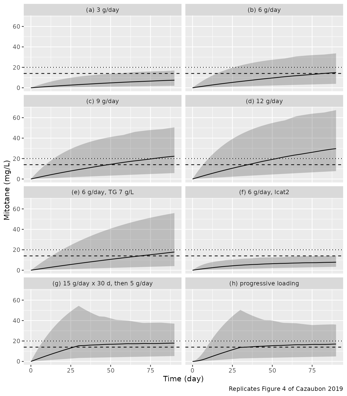
Probability of target attainment
The paper reports the percentage of simulated patients with a trough
of at least 14 mg/L (and above 20 mg/L) at three months, and at one
month for the two loading regimens (Results 3.6). The per-regimen
percentages are reproduced when the simulated patients belong to the
majority latent class (MIX_FAST_ELIM = 0), which is how the
paper’s “median covariates” simulations read: panel (f) is the same 6
g/day regimen with “plcat2 = 100%”.
pta_sim <- sim |>
  dplyr::filter(arm %in% arm_levels, time %in% c(30, 90)) |>
  dplyr::group_by(arm, time) |>
  dplyr::summarise(
    pta14 = 100 * mean(Cc >= 14), above20 = 100 * mean(Cc > 20),
    .groups = "drop"
  )
pta_paper <- tibble::tribble(
  ~arm, ~time, ~metric, ~published,
  arm_levels[1], 90, "pta14", 10,
  arm_levels[2], 90, "pta14", 55,
  arm_levels[3], 90, "pta14", 76,
  arm_levels[4], 90, "pta14", 85,
  arm_levels[5], 90, "pta14", 63.1,
  arm_levels[6], 90, "pta14", 3,
  arm_levels[7], 90, "pta14", 69,
  arm_levels[8], 90, "pta14", 65,
  arm_levels[7], 30, "pta14", 57,
  arm_levels[8], 30, "pta14", 51,
  arm_levels[2], 90, "above20", 30.4,
  arm_levels[3], 90, "above20", 58,
  arm_levels[4], 90, "above20", 73,
  arm_levels[7], 90, "above20", 42,
  arm_levels[8], 90, "above20", 39
)
pta_cmp <- pta_sim |>
  tidyr::pivot_longer(c(pta14, above20), names_to = "metric", values_to = "simulated") |>
  dplyr::inner_join(pta_paper, by = c("arm", "time", "metric")) |>
  dplyr::mutate(diff = simulated - published)
pta_cmp |>
  dplyr::mutate(metric = ifelse(metric == "pta14", ">= 14 mg/L", "> 20 mg/L")) |>
  dplyr::rename(
    Regimen = arm, "Day" = time, "Threshold" = metric,
    "Simulated (%)" = simulated, "Published (%)" = published,
    "Difference (pct points)" = diff
  ) |>
knitr::kable(digits = 1)| Regimen | Day | Threshold | Simulated (%) | Published (%) | Difference (pct points) |
|---|---|---|---|---|---|
| (a) 3 g/day | 90 | >= 14 mg/L | 8.2 | 10.0 | -1.8 |
| (b) 6 g/day | 90 | >= 14 mg/L | 53.6 | 55.0 | -1.4 |
| (b) 6 g/day | 90 | > 20 mg/L | 28.1 | 30.4 | -2.3 |
| (c) 9 g/day | 90 | >= 14 mg/L | 76.0 | 76.0 | 0.0 |
| (c) 9 g/day | 90 | > 20 mg/L | 57.1 | 58.0 | -0.9 |
| (d) 12 g/day | 90 | >= 14 mg/L | 85.7 | 85.0 | 0.7 |
| (d) 12 g/day | 90 | > 20 mg/L | 71.9 | 73.0 | -1.1 |
| (e) 6 g/day, TG 7 g/L | 90 | >= 14 mg/L | 63.3 | 63.1 | 0.2 |
| (f) 6 g/day, lcat2 | 90 | >= 14 mg/L | 2.6 | 3.0 | -0.4 |
| (g) 15 g/day x 30 d, then 5 g/day | 30 | >= 14 mg/L | 56.1 | 57.0 | -0.9 |
| (g) 15 g/day x 30 d, then 5 g/day | 90 | >= 14 mg/L | 68.4 | 69.0 | -0.6 |
| (g) 15 g/day x 30 d, then 5 g/day | 90 | > 20 mg/L | 40.3 | 42.0 | -1.7 |
| (h) progressive loading | 30 | >= 14 mg/L | 49.5 | 51.0 | -1.5 |
| (h) progressive loading | 90 | >= 14 mg/L | 65.3 | 65.0 | 0.3 |
| (h) progressive loading | 90 | > 20 mg/L | 37.2 | 39.0 | -1.8 |
All 15 published percentages are reproduced within a few percentage points. The cohort is a deterministic quadrature grid, so the only error on our side is the 14-node discretisation; the paper’s figures come from 1000 simulated patients and carry a Monte-Carlo standard error of about 1.5 percentage points. A mis-transcribed clearance, volume, bioavailability or covariate exponent moves these percentages by tens of points.
External evaluation (Kerkhofs)
The paper simulated the mean cumulative doses of the Kerkhofs et al. low- and high-dose groups (272 g and 440 g over 12 weeks) and reported simulated median week-12 plasma levels of 8.2 and 13.3 mg/L, and 14.6% and 46.5% of patients at or above 14 mg/L (Results 3.5). Here the cumulative dose is given as a constant daily dose over 84 days.
kerk <- sim |>
  dplyr::filter(grepl("Kerkhofs", arm), time == 84) |>
  dplyr::group_by(arm) |>
  dplyr::summarise(median_Cc = median(Cc), pta14 = 100 * mean(Cc >= 14), .groups = "drop") |>
  dplyr::mutate(
    published_median = c(13.3, 8.2)[match(arm, c("Kerkhofs high dose (440 g / 84 d)", "Kerkhofs low dose (272 g / 84 d)"))],
    published_pta14 = c(46.5, 14.6)[match(arm, c("Kerkhofs high dose (440 g / 84 d)", "Kerkhofs low dose (272 g / 84 d)"))]
  )
kerk |>
  dplyr::rename(
    Group = arm, "Simulated median (mg/L)" = median_Cc, "Published simulated median (mg/L)" = published_median,
    "Simulated PTA (%)" = pta14, "Published simulated PTA (%)" = published_pta14
  ) |>
knitr::kable(digits = 1)| Group | Simulated median (mg/L) | Simulated PTA (%) | Published simulated median (mg/L) | Published simulated PTA (%) |
|---|---|---|---|---|
| Kerkhofs high dose (440 g / 84 d) | 12.4 | 41.3 | 13.3 | 46.5 |
| Kerkhofs low dose (272 g / 84 d) | 7.7 | 10.7 | 8.2 | 14.6 |
The medians agree within about 7%. The simulated PTAs are 4-5 points below the paper’s; the paper does not state how the cumulative dose was spread over the 12 weeks (Kerkhofs et al. titrated doses upward), which moves the week-12 trough.
PKNCA validation
A single 1 g dose is simulated for the same 196-subject grid (majority class, median covariates) and sampled for 600 days (about 7 half-lives). The paper reports no NCA, so the NCA is compared with the model’s own closed form for the typical patient: AUC0-inf = F x Dose / CL = 5 mg.day/L and t1/2 = ln(2) V / CL = 88.1 days (medians over the symmetric eta grid equal the typical values).
sd_rows <- dplyr::bind_rows(
  data.frame(time = 0, amt = 1000, evid = 1L, cmt = "depot"),
  data.frame(
    time = c(0, 0.02, 0.05, 0.1, 0.2, 0.3, 0.5, 1, 2, 4, 7, seq(14, 600, by = 14)),
    amt = 0, evid = 0L, cmt = "central"
  )
)
sd_events <- merge(grid, sd_rows, by = NULL)
sd_events$id <- sd_events$sid
sd_events$arm <- "1 g single dose"
sd_events$TRIG <- 1.56
sd_events$HDLC <- 0.65
sd_events$MIX_FAST_ELIM <- 0
sd_events <- sd_events[order(sd_events$id, sd_events$time, -sd_events$evid), ]
sim_sd <- rxode2::rxSolve(mod,
  events = sd_events, omega = NA, sigma = NA, keep = "arm",
  rtol = 1e-10, atol = 1e-12, returnType = "data.frame"
)
conc <- sim_sd |>
  dplyr::filter(!is.na(Cc)) |>
  dplyr::select(id, time, Cc, arm)
dose <- sd_events |>
  dplyr::filter(evid == 1L) |>
  dplyr::select(id, time, amt, arm)
o_conc <- PKNCA::PKNCAconc(conc, Cc ~ time | arm + id)
o_dose <- PKNCA::PKNCAdose(dose, amt ~ time | arm + id)
intervals <- data.frame(start = 0, end = Inf, cmax = TRUE, tmax = TRUE, aucinf.obs = TRUE, half.life = TRUE)
nca <- PKNCA::pk.nca(PKNCA::PKNCAdata(o_conc, o_dose, intervals = intervals))
reference <- data.frame(
  arm = "1 g single dose",
  aucinf.obs = 0.35 * 1000 / 70,
  half.life = log(2) * 8900 / 70
)
cmp <- ncaComparisonTable(nca, reference,
  by = "arm", params = c("aucinf.obs", "half.life"),
  units = c(aucinf.obs = "mg*day/L", half.life = "day")
)
knitr::kable(cmp)| NCA parameter | arm | Reference | Simulated | % diff |
|---|---|---|---|---|
| AUC0-∞ (obs) (mg*day/L) | 1 g single dose | 5 | 5 | +0.0% |
| t½ (day) | 1 g single dose | 88.1 | 88.1 | +0.0% |
Assumptions and deviations
- Omega scale. Monolix reports each random effect as the standard deviation omega of the log-normal eta; Table 2 prints these as percentages (90.4% and 29.3%). They are encoded as variances omega^2 (0.817 and 0.0858). The alternative reading (a CV% converted by log(1 + CV^2)) gives variances of 0.597 and 0.0824. The target-attainment percentages do not discriminate the two readings well (they differ by 1-4 points), so the Monolix convention is used.
-
Residual-error form. The paper reports a combined
error with a = 1.06 mg/L and b = 0.17 but not which Monolix combined
form was used; the Monolix default
combined1(SD = a + b f) is encoded (combined1()). - Signs of the covariate exponents. The PDF’s text layer loses the minus signs; the typeset page prints beta_HDL = -0.344 and beta_Tg = -0.526 with negative bootstrap intervals, and the Discussion states that higher Tg and HDL lower clearance.
-
Latent class in simulations. The latent-class
indicator is supplied as the covariate
MIX_FAST_ELIM(1 = lcat2, the ultrafast subpopulation). For a population simulation, draw it as Bernoulli(0.115). The paper’s Figure 4 simulations reproduce withMIX_FAST_ELIM = 0, except panel (f). - Dose split. The paper’s patients took the daily dose in 2-4 administrations and the simulation software’s split is not stated; three equal daily administrations are used. With ka = 24/day and a ~90-day half-life, the trough is insensitive to the split.
- Units. Time is in days, CL in L/day (the abstract’s “L h-1” is a typo; Table 2 gives L day-1, and the Discussion compares it to Arshad’s 75 L/day). TRIG and HDLC are in g/L, as in Table 1.
- Time-varying covariates. The paper used each patient’s median lipid values (Methods 2.5), so TRIG and HDLC are time-fixed per subject.