Vonoprazan PBPK-PD in rats, dogs and humans (Kong 2020)
Source:vignettes/articles/Kong_2020_vonoprazan_pbpk.Rmd
Kong_2020_vonoprazan_pbpk.RmdModel and source
Kong et al. (2020) built one whole-body physiologically based
pharmacokinetic-pharmacodynamic (PBPK-PD) structure for vonoprazan, a
potassium-competitive acid blocker. They parameterised it from in vitro
data for the rat, extrapolated it to the dog, and then to a 70-kg human.
nlmixr2lib carries the three species as three models that share an
identical model() block and differ only in
ini() values:
mod_rat   <- readModelDb("Kong_2020_vonoprazan_rat_pbpk")
mod_dog   <- readModelDb("Kong_2020_vonoprazan_dog_pbpk")
mod_human <- readModelDb("Kong_2020_vonoprazan_human_pbpk")- Citation: Kong WM, Sun BB, Wang ZJ, Zheng XK, Zhao KJ, Chen Y, Zhang JX, Liu PH, Zhu L, Xu RJ, Li P, Liu L, Liu XD. Physiologically based pharmacokinetic-pharmacodynamic modeling for prediction of vonoprazan pharmacokinetics and its inhibition on gastric acid secretion following intravenous/oral administration to rats, dogs and humans. Acta Pharmacol Sin. 2020;41(6):852-865. doi:10.1038/s41401-019-0353-2. Equations 2-22 of the paper; physiology from Table 1; drug-specific values from the Methods and Results text; ODE routing from the WinNonlin ‘Mode code of human following oral administration’ listing in the Supplementary Information.
- Article: https://doi.org/10.1038/s41401-019-0353-2 (open access, PMC7468366)
- Description (human): PBPK-PD (whole-body, perfusion-limited, WinNonlin 8.1). Vonoprazan disposition and gastric-acid antisecretory effect in a typical 70-kg adult after oral dosing, extrapolated by Kong et al. (2020) from in vitro metabolism (hepatic microsomes), permeability (Caco-2) and rat tissue-distribution data. Thirteen perfusion-limited tissues plus venous and arterial blood pools; the stomach wall (the target organ) is permeability-limited with a vascular and an extravascular space. Oral doses enter the stomach lumen and transit a five-segment gut lumen (duodenum, jejunum, ileum absorb; cecum and colon do not) into per-segment gut-wall compartments. Hepatic Michaelis-Menten metabolism of unbound drug is scaled from microsomes by a physiologically based scaling factor, and an allometrically scaled linear ‘other’ clearance acts on venous blood. The PD layer drives an H+/K+-ATPase inhibition state from the unbound extravascular stomach concentration (dI/dt = k * fu * C2 * (Imax - I) - kd * I) and reports intragastric pH as basal pH + I. Deterministic typical-value model with no IIV. Companion rat and dog models: modellib(‘Kong_2020_vonoprazan_rat_pbpk’) and modellib(‘Kong_2020_vonoprazan_dog_pbpk’).
Structure (paper Figure 1 and Equations 2-22):
- Thirteen tissues (lung, heart, brain, muscle, adipose, skin, kidney, spleen, liver, rest of body, and the gut-wall segments) are perfusion-limited (Eq 2), with venous (Eq 3) and arterial (Eq 6) blood pools and the lung between them (Eq 7).
- The liver (Eqs 8-11) receives hepatic-artery flow plus portal
inflow. It clears unbound drug by Michaelis-Menten M-I formation, which
is scaled from liver microsomes by the physiologically based scaling
factor (PBSF). A separate linear
CLother(Eqs 4-5) acts on venous blood. - The stomach wall, which is the target organ, is permeability-limited
(Eqs 12-13). It has a vascular space
V1and an extravascular spaceV2, exchanging through the permeability-surface productPS(Eq 14). - Oral doses enter the stomach lumen (Eq 15), transit five gut-lumen
segments (Eq 16) and are absorbed from the duodenum, jejunum and ileum
at
ka,i = 2 Peff / r_i(Eqs 17-19) into gut-wall compartments (Eq 20). - PD (Eq 22):
dI/dt = k * fu * C2 * (Imax - I) - kd * I, withk = kd / KI.Iis the increase in gastric pH (rat, human) or the percent inhibition of acid output (dog).
Population
- Rat: female Sprague-Dawley rats of 200-250 g (0.25 kg reference). There were 25 animals in five pharmacokinetic groups (intravenous 0.5, 1 and 2 mg/kg; oral 2 mg/kg; intravenous 1 mg/kg daily for 7 days) and 15 in a tissue-distribution study. The gastric-pH comparison data came from the literature (histamine-stimulated anaesthetised rats).
- Dog: eight beagles (4 female, 4 male, 7-10 kg; 8.5 kg reference) in a four-period crossover (intravenous 0.15, 0.3 and 0.6 mg/kg; oral 0.6 mg/kg) followed by 7 days of intravenous dosing. The acid-output comparison data came from the literature (histamine-stimulated Heidenhain-pouch dogs).
- Human: a 70-kg reference adult. The comparison data are published healthy-volunteer studies from Japan and the UK (single oral doses of 5-40 mg and 10-40 mg once daily for 7 days).
This is a bottom-up prediction model rather than a population fit.
The only parameter fitted to in vivo data is the rat stomach
PS (0.6 mL/min), which was fitted to rat stomach
concentrations. The model has no between-subject variability. The
paper’s human visual predictive check estimated variances on CLliver, fu
and k but did not report them. The same information is available
programmatically as
rxode2::rxode(mod_human)$population.
Source trace
Every ini() value carries an in-file comment that points
to its source. The table below collects the drug-specific values. The
organ volumes, blood flows and Kt:p values are transcribed
column by column from Table 1 (rat 0.25 kg, dog 8.5 kg, human 70
kg).
| Parameter | Rat | Dog | Human | Source |
|---|---|---|---|---|
Organ volumes, blood flows, Kt:p, radii
r1-r3, transit k0-k5
|
Table 1 | Table 1 | Table 1 | Table 1 |
fu |
0.32 | 0.17 | 0.15 | Methods, Kt:p scaling paragraph |
bp (Rb) |
0.91 | 0.91 | 0.91 | Methods, Eq 2 text |
vmax (nmol/min/mg) |
1.50 | 0.16 | 0.24 | Results, microsomal M-I formation |
km (uM) |
12.94 | 90.97 | 13.60 | Results, microsomal M-I formation |
pbsf (mg protein/body) |
409.92 | 16592.7 | 82472 | Methods, Eq 4 text |
cl_other (mL/min) |
25 | 150 | 616 | Methods, Eq 5 text; Results |
ps_stomach (mL/min) |
0.6 (fitted) | 6.37 | 26.17 | Results; Eq 14 |
v_vp_stomach / v_ev_stomach (mL) |
0.2 / 0.9 | 4.6 / 19.4 | 25.6 / 134.4 | Methods, Eqs 12-13 text |
peff (cm/min) |
0.002 | 0.008 | 0.008 | Methods, Eqs 18-19 text; Results |
kd (1/min) |
0.00246 | 0.00246 | 0.00246 | Methods, Eq 22 text (dissociation t1/2 4.7 h) |
ki (uM) |
0.035 | 0.035 | 0.035 | Methods, Eq 21 text (KI = 35 nM) |
imax |
4.0 pH | 100 % | 5.0 pH | Results, per species |
ph_basal (pH) |
2.0 | n/a | 2.0 | Results, per species |
mw (g/mol) |
345.08 | 345.08 | 345.08 | Supplement code tvKm = 4693.14 ng/mL divided by Km
13.60 uM |
| ODE routing into liver and venous blood | Supplementary “Mode code of human following oral administration” |
The derived hepatic-artery flow is
q_ha = q_liver - q_stomach - q_spleen - sum(q_gw). It gives
300 mL/min for the human, which is the supplement’s
tvQliver. The Table 1 liver Kt:p values
already include the Eq 11 extraction-ratio correction: applying Eqs
10-11 to the rat value scaled by fu returns the tabulated
dog and human 2.89.
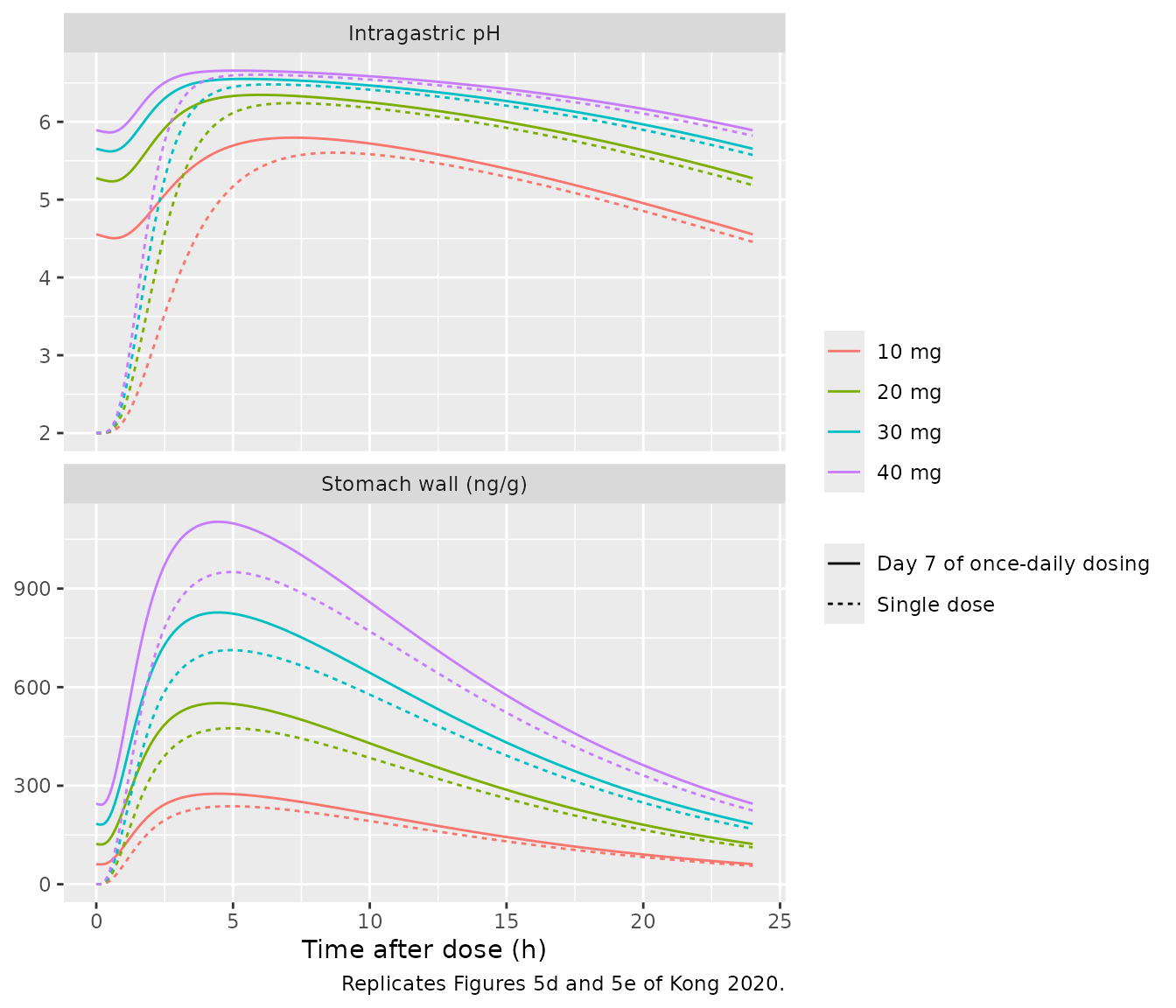
Human: oral single and multiple doses (Table 4, Figure 5)
# One typical 70-kg adult per regimen; deterministic model, no IIV.
human_regimen <- function(dose, n_doses, id) {
  ev <- if (n_doses == 1) {
    rxode2::et(amt = dose, cmt = "stomach")
  } else {
    rxode2::et(amt = dose, cmt = "stomach", ii = 1440, addl = n_doses - 1)
  }
  ev <- rxode2::et(ev, seq(0, 1440 * n_doses, by = 5))
  d <- as.data.frame(ev)
  d$id <- id
  d$treatment <- sprintf("%g mg %s", dose, if (n_doses == 1) "single" else "x 7 days")
  d
}
human_events <- bind_rows(
  human_regimen(10, 1, 1), human_regimen(20, 1, 2),
  human_regimen(30, 1, 3), human_regimen(40, 1, 4),
  human_regimen(10, 7, 5), human_regimen(20, 7, 6),
  human_regimen(30, 7, 7), human_regimen(40, 7, 8)
)
stopifnot(!anyDuplicated(unique(human_events[, c("id", "time", "evid")])))
sim_human <- rxode2::rxSolve(mod_human, events = human_events, keep = "treatment") |>
  as.data.frame()
#> Warning: multi-subject simulation without without 'omega'
sim_human |>
  filter(grepl("single", treatment), time <= 1440) |>
  ggplot(aes(time / 60, Cc, colour = treatment)) +
  geom_line() +
  scale_y_log10() +
  labs(
    x = "Time after dose (h)", y = "Plasma vonoprazan (ng/mL)", colour = NULL,
    caption = "Replicates Figure 5a of Kong 2020 (model predictions only)."
  )
#> Warning in scale_y_log10(): log-10 transformation introduced infinite values.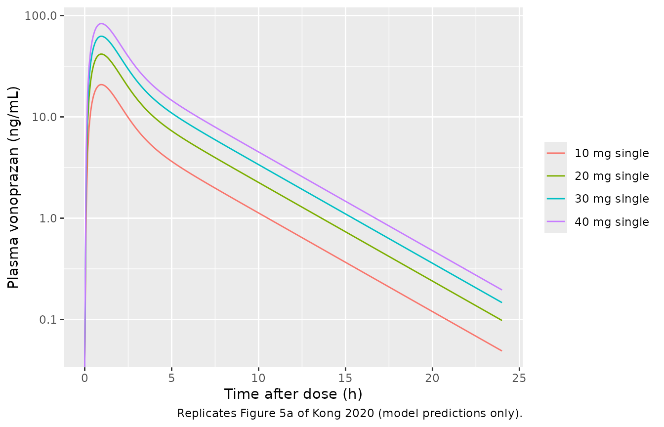
sim_human |>
  filter(grepl("single", treatment) | time >= 1440 * 6) |>
  mutate(
    tad = ifelse(grepl("single", treatment), time, time - 1440 * 6),
    regimen = ifelse(grepl("single", treatment), "Single dose", "Day 7 of once-daily dosing"),
    dose = sub(" .*", " mg", treatment)
  ) |>
  filter(tad <= 1440) |>
  select(tad, regimen, dose, `Stomach wall (ng/g)` = Cstomach, `Intragastric pH` = gastric_ph) |>
  pivot_longer(c(`Stomach wall (ng/g)`, `Intragastric pH`)) |>
  ggplot(aes(tad / 60, value, colour = dose, linetype = regimen)) +
  geom_line() +
  facet_wrap(~name, scales = "free_y", ncol = 1) +
  labs(
    x = "Time after dose (h)", y = NULL, colour = NULL, linetype = NULL,
    caption = "Replicates Figures 5d and 5e of Kong 2020."
  )
PKNCA against the paper’s predicted Table 4 values
Table 4 prints both the observed human NCA and the paper’s own model
predictions. The packaged model is compared with the
predicted columns, because those are the output of the
same model structure. AUC0-tn is taken over 0-24 h after
the (last) dose. Table 4 prints AUC in minug/mL; it is converted to
minng/mL here.
nca_conc <- sim_human |>
  filter(!is.na(Cc)) |>
  mutate(
    day7 = !grepl("single", treatment),
    time_nca = ifelse(day7, time - 1440 * 6, time)
  ) |>
  filter(time_nca >= 0, time_nca <= 1440) |>
  select(id, treatment, time = time_nca, Cc)
nca_dose <- human_events |>
  filter(evid == 1) |>
  mutate(time = ifelse(grepl("single", treatment), time, time - 1440 * 6)) |>
  filter(time == 0) |>
  select(id, treatment, time, amt)

human_nca <- PKNCA::pk.nca(PKNCA::PKNCAdata(
  PKNCA::PKNCAconc(nca_conc, Cc ~ time | treatment + id),
  PKNCA::PKNCAdose(nca_dose, amt ~ time | treatment + id),
  intervals = data.frame(start = 0, end = 1440, cmax = TRUE, tmax = TRUE, auclast = TRUE)
))

human_pub <- tibble::tribble(
  ~treatment,        ~cmax, ~tmax, ~auclast,
  "10 mg single",    20.79, 55,    4.01 * 1000,
  "20 mg single",    41.59, 55,    8.02 * 1000,
  "30 mg single",    62.40, 55,    12.04 * 1000,
  "40 mg single",    83.22, 55,    16.05 * 1000,
  "10 mg x 7 days",  20.83, 55,    4.02 * 1000,
  "20 mg x 7 days",  41.67, 55,    8.04 * 1000,
  "30 mg x 7 days",  62.52, 55,    12.06 * 1000,
  "40 mg x 7 days",  83.38, 55,    16.09 * 1000
)
human_cmp <- nlmixr2lib::ncaComparisonTable(
  human_nca, human_pub,
  by = "treatment",
  units = c(cmax = "ng/mL", tmax = "min", auclast = "min*ng/mL"),
  tolerance_pct = 20
)
knitr::kable(human_cmp, caption = "Human: simulated vs. Kong 2020 Table 4 predicted values. * > 20% difference.")| NCA parameter | treatment | Reference | Simulated | % diff |
|---|---|---|---|---|
| Cmax (ng/mL) | 10 mg single | 20.8 | 20.8 | +0.1% |
| Cmax (ng/mL) | 20 mg single | 41.6 | 41.6 | +0.1% |
| Cmax (ng/mL) | 30 mg single | 62.4 | 62.5 | +0.1% |
| Cmax (ng/mL) | 40 mg single | 83.2 | 83.3 | +0.1% |
| Cmax (ng/mL) | 10 mg x 7 days | 20.8 | 20.9 | +0.1% |
| Cmax (ng/mL) | 20 mg x 7 days | 41.7 | 41.7 | +0.1% |
| Cmax (ng/mL) | 30 mg x 7 days | 62.5 | 62.6 | +0.1% |
| Cmax (ng/mL) | 40 mg x 7 days | 83.4 | 83.5 | +0.1% |
| Tmax (min) | 10 mg single | 55 | 55 | +0.0% |
| Tmax (min) | 20 mg single | 55 | 55 | +0.0% |
| Tmax (min) | 30 mg single | 55 | 55 | +0.0% |
| Tmax (min) | 40 mg single | 55 | 55 | +0.0% |
| Tmax (min) | 10 mg x 7 days | 55 | 55 | +0.0% |
| Tmax (min) | 20 mg x 7 days | 55 | 55 | +0.0% |
| Tmax (min) | 30 mg x 7 days | 55 | 55 | +0.0% |
| Tmax (min) | 40 mg x 7 days | 55 | 55 | +0.0% |
| AUClast (min*ng/mL) | 10 mg single | 4010 | 4010 | -0.1% |
| AUClast (min*ng/mL) | 20 mg single | 8020 | 8010 | -0.1% |
| AUClast (min*ng/mL) | 30 mg single | 12000 | 12000 | -0.1% |
| AUClast (min*ng/mL) | 40 mg single | 16000 | 16000 | -0.1% |
| AUClast (min*ng/mL) | 10 mg x 7 days | 4020 | 4020 | -0.0% |
| AUClast (min*ng/mL) | 20 mg x 7 days | 8040 | 8040 | -0.0% |
| AUClast (min*ng/mL) | 30 mg x 7 days | 12100 | 12100 | +0.0% |
| AUClast (min*ng/mL) | 40 mg x 7 days | 16100 | 16100 | -0.0% |
human_diff <- as.numeric(gsub("[^0-9.eE-]", "", human_cmp[["% diff"]]))
# Deterministic model with the same structure as the paper's: the paper's
# predictions are reproduced to within 0.1% (the 5-min grid limits Tmax
# resolution, which lands exactly on the paper's 55 min).
stopifnot(all(abs(human_diff) < 2))
The published human predictions are reproduced. The paper reports its
own model’s predicted Cmax as roughly twice the observed
values, and underpredicts t1/2 (about 191 min predicted
against 350-500 min observed) throughout Table 4. That is a property of
the published model, not of this implementation.
Rat: oral pharmacokinetics, intravenous stomach concentration and gastric pH (Table 2, Figure 2)
rat_wt <- 0.25
rat_regimen <- function(dose_mgkg, route, id, tend) {
  cmt <- if (route == "iv") "venous" else "stomach"
  ev <- rxode2::et(amt = dose_mgkg * rat_wt, cmt = cmt) |> rxode2::et(seq(0, tend, by = 0.5))
  d <- as.data.frame(ev)
  d$id <- id
  d$treatment <- sprintf("%s %g mg/kg", route, dose_mgkg)
  d
}
rat_events <- bind_rows(
  rat_regimen(2, "oral", 1, 240),
  rat_regimen(0.5, "iv", 2, 600),
  rat_regimen(0.7, "iv", 3, 600),
  rat_regimen(1.0, "iv", 4, 600)
)
sim_rat <- rxode2::rxSolve(mod_rat, events = rat_events, keep = "treatment") |> as.data.frame()
#> Warning: multi-subject simulation without without 'omega'

rat_oral_nca <- PKNCA::pk.nca(PKNCA::PKNCAdata(
  PKNCA::PKNCAconc(filter(sim_rat, treatment == "oral 2 mg/kg", !is.na(Cc)) |>
    select(id, treatment, time, Cc), Cc ~ time | treatment + id),
  PKNCA::PKNCAdose(filter(rat_events, evid == 1, treatment == "oral 2 mg/kg") |>
    select(id, treatment, time, amt), amt ~ time | treatment + id),
  intervals = data.frame(start = 0, end = 240, cmax = TRUE, tmax = TRUE, auclast = TRUE)
))
rat_cmp <- nlmixr2lib::ncaComparisonTable(
  rat_oral_nca,
  tibble::tibble(treatment = "oral 2 mg/kg", cmax = 35.52, tmax = 55.5, auclast = 3.90 * 1000),
  by = "treatment",
  units = c(cmax = "ng/mL", tmax = "min", auclast = "min*ng/mL")
)
knitr::kable(rat_cmp, caption = "Rat oral 2 mg/kg: simulated vs. Kong 2020 Table 2 predicted values (AUC0-240 min).")| NCA parameter | treatment | Reference | Simulated | % diff |
|---|---|---|---|---|
| Cmax (ng/mL) | oral 2 mg/kg | 35.5 | 35.6 | +0.2% |
| Tmax (min) | oral 2 mg/kg | 55.5 | 55.5 | +0.0% |
| AUClast (min*ng/mL) | oral 2 mg/kg | 3900 | 3910 | +0.1% |
stopifnot(all(abs(as.numeric(gsub("[^0-9.eE-]", "", rat_cmp[["% diff"]]))) < 3))
sim_rat |>
  filter(grepl("iv", treatment)) |>
  select(time, treatment, `Stomach wall (ng/g)` = Cstomach, `Gastric perfusate pH` = gastric_ph) |>
  pivot_longer(-c(time, treatment)) |>
  ggplot(aes(time / 60, value, colour = treatment)) +
  geom_line() +
  facet_wrap(~name, scales = "free_y", ncol = 1) +
  labs(
    x = "Time after dose (h)", y = NULL, colour = NULL,
    caption = "Replicates Figures 2e and 2f of Kong 2020."
  )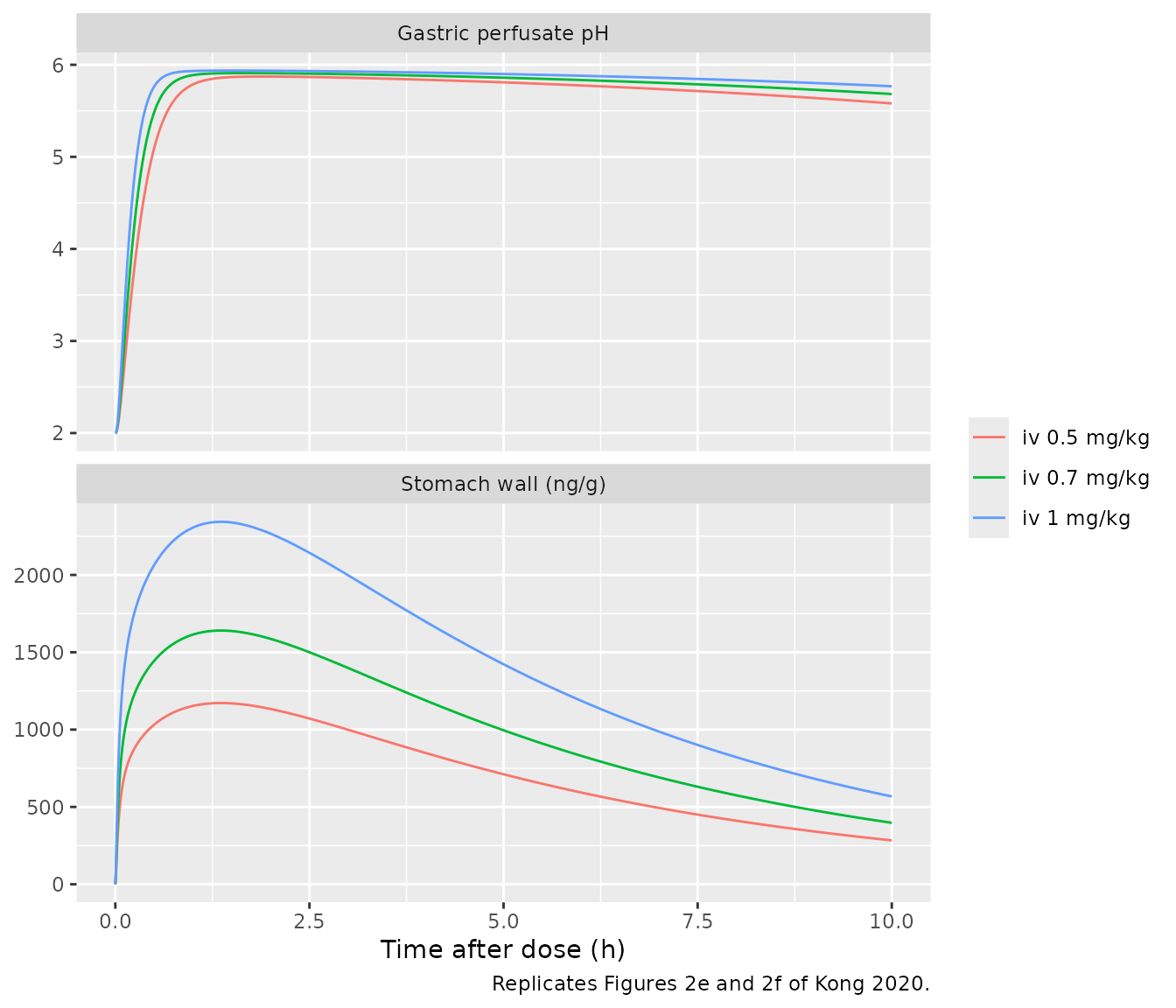
The Results text prints stomach and plasma concentrations 5 h after intravenous dosing:
rat_5h <- sim_rat |>
  filter(time == 300, treatment %in% c("iv 0.7 mg/kg", "iv 1 mg/kg")) |>
  transmute(treatment,
    stomach_sim = Cstomach, stomach_paper = c(1043, 1490),
    plasma_sim = Cc, plasma_paper = c(0.25, 0.35)
  )
knitr::kable(rat_5h, digits = 3, caption = "Rat, 5 h after intravenous dosing: simulated vs. Results text.")| treatment | stomach_sim | stomach_paper | plasma_sim | plasma_paper |
|---|---|---|---|---|
| iv 0.7 mg/kg | 995.698 | 1043 | 0.202 | 0.25 |
| iv 1 mg/kg | 1422.488 | 1490 | 0.289 | 0.35 |
# Known deviation, see Assumptions: the paper's rat intravenous simulations
# are not reproduced exactly. Stomach is ~5% and plasma ~18% below the
# printed values; the gate pins the size of that gap so a regression shows.
stopifnot(
  all(abs(rat_5h$stomach_sim / rat_5h$stomach_paper - 1) < 0.10),
  all(abs(rat_5h$plasma_sim / rat_5h$plasma_paper - 1) < 0.25)
)
Dog: oral pharmacokinetics and Heidenhain-pouch acid output (Table 3, Figure 4)
dog_wt <- 8.5
dog_regimen <- function(dose_mgkg, id, tend, by) {
  ev <- rxode2::et(amt = dose_mgkg * dog_wt, cmt = "stomach") |> rxode2::et(seq(0, tend, by = by))
  d <- as.data.frame(ev)
  d$id <- id
  d$treatment <- sprintf("oral %g mg/kg", dose_mgkg)
  d
}
dog_events <- bind_rows(
  dog_regimen(0.6, 1, 300, 0.5),
  dog_regimen(0.1, 2, 1440, 5),
  dog_regimen(0.3, 3, 1440, 5),
  dog_regimen(1.0, 4, 1440, 5)
)
sim_dog <- rxode2::rxSolve(mod_dog, events = dog_events, keep = "treatment") |> as.data.frame()
#> Warning: multi-subject simulation without without 'omega'

dog_oral_nca <- PKNCA::pk.nca(PKNCA::PKNCAdata(
  PKNCA::PKNCAconc(filter(sim_dog, treatment == "oral 0.6 mg/kg", !is.na(Cc)) |>
    select(id, treatment, time, Cc), Cc ~ time | treatment + id),
  PKNCA::PKNCAdose(filter(dog_events, evid == 1, treatment == "oral 0.6 mg/kg") |>
    select(id, treatment, time, amt), amt ~ time | treatment + id),
  intervals = data.frame(start = 0, end = 300, cmax = TRUE, tmax = TRUE, auclast = TRUE)
))
dog_cmp <- nlmixr2lib::ncaComparisonTable(
  dog_oral_nca,
  tibble::tibble(treatment = "oral 0.6 mg/kg", cmax = 145.73, tmax = 43, auclast = 16.26 * 1000),
  by = "treatment",
  units = c(cmax = "ng/mL", tmax = "min", auclast = "min*ng/mL")
)
knitr::kable(dog_cmp, caption = "Dog oral 0.6 mg/kg: simulated vs. Kong 2020 Table 3 predicted values (AUC0-300 min).")| NCA parameter | treatment | Reference | Simulated | % diff |
|---|---|---|---|---|
| Cmax (ng/mL) | oral 0.6 mg/kg | 146 | 146 | -0.0% |
| Tmax (min) | oral 0.6 mg/kg | 43 | 43 | +0.0% |
| AUClast (min*ng/mL) | oral 0.6 mg/kg | 16300 | 16300 | -0.0% |
stopifnot(all(abs(as.numeric(gsub("[^0-9.eE-]", "", dog_cmp[["% diff"]]))) < 3))
sim_dog |>
  filter(treatment != "oral 0.6 mg/kg") |>
  select(time, treatment, `Stomach wall (ng/g)` = Cstomach, `Acid output (% of predose)` = acid_output) |>
  pivot_longer(-c(time, treatment)) |>
  ggplot(aes(time / 60, value, colour = treatment)) +
  geom_line() +
  facet_wrap(~name, scales = "free_y", ncol = 1) +
  labs(
    x = "Time after dose (h)", y = NULL, colour = NULL,
    caption = "Replicates Figures 4e and 4f of Kong 2020."
  )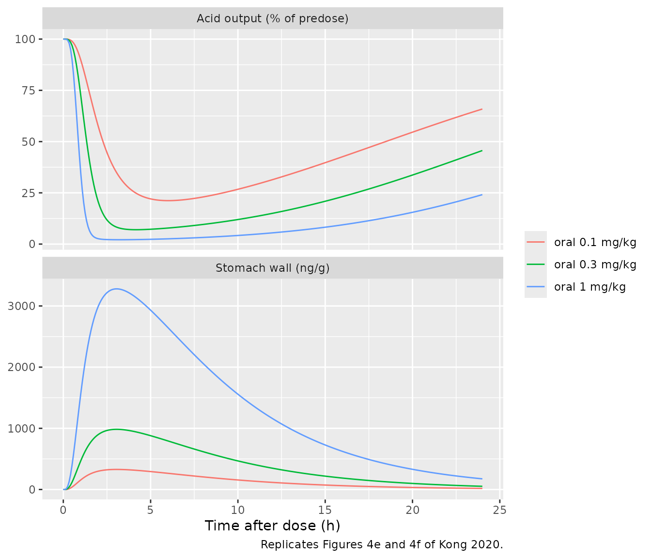
The Results text prints the 24-h values after 0.3 and 1.0 mg/kg:
dog_24h <- sim_dog |>
  filter(time == 1440, treatment %in% c("oral 0.3 mg/kg", "oral 1 mg/kg")) |>
  transmute(treatment,
    stomach_sim = Cstomach, stomach_paper = c(52.31, 174.39),
    plasma_sim = Cc, plasma_paper = c(0.0016, 0.0055),
    acid_sim = acid_output, acid_paper = c(48, 26)
  )
knitr::kable(dog_24h, digits = 4, caption = "Dog, 24 h after oral dosing: simulated vs. Results text.")| treatment | stomach_sim | stomach_paper | plasma_sim | plasma_paper | acid_sim | acid_paper |
|---|---|---|---|---|---|---|
| oral 0.3 mg/kg | 52.3110 | 52.31 | 0.0016 | 0.0016 | 45.6426 | 48 |
| oral 1 mg/kg | 174.3744 | 174.39 | 0.0055 | 0.0055 | 24.1253 | 26 |
stopifnot(
  # Stomach concentrations are printed to 4-5 significant figures and match.
  all(abs(dog_24h$stomach_sim / dog_24h$stomach_paper - 1) < 0.01),
  # Plasma is printed to 2 significant figures.
  all(abs(dog_24h$plasma_sim / dog_24h$plasma_paper - 1) < 0.05),
  # Acid output: 2-3 percentage points below the printed values (see Assumptions).
  all(abs(dog_24h$acid_sim - dog_24h$acid_paper) < 5)
)
Intravenous predictions (Tables 2 and 3)
iv_auc <- function(mod, wt, dose_mgkg, tn) {
  # Log-spaced grid: the bolus lands in a small venous volume, so a coarse
  # linear grid overstates the trapezoidal AUC over the first minute.
  ev <- rxode2::et(amt = dose_mgkg * wt, cmt = "venous") |>
    rxode2::et(c(0, exp(seq(log(1e-3), log(tn), length.out = 3000))))
  s <- as.data.frame(rxode2::rxSolve(mod, events = ev))
  sum(diff(s$time) * (head(s$Cc, -1) + tail(s$Cc, -1)) / 2) / 1000
}
iv_tab <- tibble::tribble(
  ~species, ~dose_mgkg, ~auc_paper,
  "rat", 0.5, 3.21,
  "rat", 1.0, 6.42,
  "dog", 0.15, 7.31,
  "dog", 0.3, 14.62
) |>
  rowwise() |>
  mutate(auc_sim = if (species == "rat") {
    iv_auc(mod_rat, rat_wt, dose_mgkg, 240)
  } else {
    iv_auc(mod_dog, dog_wt, dose_mgkg, 300)
  }) |>
  ungroup() |>
  mutate(ratio = auc_sim / auc_paper)
iv_tab |>
  rename(
    "Species" = species, "IV dose (mg/kg)" = dose_mgkg,
    "Paper predicted AUC0-tn (min*ug/mL)" = auc_paper,
    "Simulated AUC0-tn (min*ug/mL)" = auc_sim, "Simulated / paper" = ratio
  ) |>
knitr::kable(digits = 2, caption = "Intravenous AUC: simulated vs. the paper's predicted values (known deviation).")| Species | IV dose (mg/kg) | Paper predicted AUC0-tn (min*ug/mL) | Simulated AUC0-tn (min*ug/mL) | Simulated / paper |
|---|---|---|---|---|
| rat | 0.50 | 3.21 | 4.06 | 1.26 |
| rat | 1.00 | 6.42 | 8.12 | 1.26 |
| dog | 0.15 | 7.31 | 4.28 | 0.59 |
| dog | 0.30 | 14.62 | 8.55 | 0.59 |
Assumptions and deviations
-
ODE routing follows the supplement code, not a
mass-conserving reading of Eq 8. The supplementary WinNonlin
listing for the human oral model does two things that a textbook PBPK
would not. First, it passes the stomach vascular outflow to the liver as
Qstomach * C1 / (Kp,stomach / Rb)rather thanQstomach * C1. Second, it routes only the three absorbing gut-wall segments (duodenum, jejunum, ileum) to the liver, so the venous outflow of the cecum and colon walls is not returned to the circulation. Both lose drug and so act as additional elimination pathways. The maintainers kept this routing because it reproduces the paper’s published oral predictions for all three species exactly: human Table 4, rat and dog Tables 2 and 3, and the dog 24-h stomach and plasma values. A mass-conserving variant, with stomach outflowQstomach * C1and cecum and colon routed to the liver, gives a human 20 mg AUC of about 11.0 rather than the published 8.02 minug/mL, and a dog oral AUC of about 27.5 rather than 16.26 minug/mL. The same routing is applied to the rat and dog models, for which no code was published. - Intravenous predictions are not reproduced. The rat intravenous AUCs are about 26% above Table 2’s predictions, the rat 5-h plasma values about 18% below the Results text, and the dog intravenous AUCs about 42% below Table 3’s. The maintainers found that the dog intravenous predictions (AUC 14.42 vs. 14.62 min*ug/mL at 0.3 mg/kg; CL 17.6 vs. 18.04 mL/min/kg) are reproduced if the cecum and colon walls drain to the liver. That same change breaks the exact match of the dog oral prediction, which suggests the authors ran intravenous simulations with a differently routed model. No single routing reproduces both routes, and no rat variant tried reproduced Table 2’s intravenous values. The packaged models therefore follow the one published code listing, and the intravenous gap is pinned in the check above rather than tuned away.
- The paper’s summary “predicted CL 874 mL/min and Vss 228 L” for the human is not reproduced by any routing variant. The code-literal model has an intravenous plasma clearance of about 1020 mL/min. The paper does not say how these two summary numbers were computed. They are not used as a gate.
-
Molecular weight. The paper does not print one. The
supplement code expresses
Kmas 4693.14 ng/mL against the printed 13.60 uM, which implies 345.08 g/mol; that value converts uM to ng/mL for both the hepatic Michaelis-Menten term and the PD binding term. The formula weight of vonoprazan free base (C17H16FN3O2S) is 345.39 g/mol, 0.09% different. -
Vmax. The supplement code carries
Vmax = 83.54ng/min/mg protein, which is 0.242 nmol/min/mg at 345.08 g/mol. The packaged human model uses the 0.24 nmol/min/mg printed in the Results, and the 0.8% difference has no visible effect on the Table 4 comparison.PSis 26.17 mL/min from the Results text; the code carries the rounded 26.2. -
Liver
Kt:p. Table 1 liver values already include the Eq 11 extraction-ratio correction (they are internally consistent with Eqs 10-11 applied to the rat value), so they are used as printed, as the supplement code does. -
Rat and dog cecum and colon transit
(
k4,k5) are “ND” in Table 1 and are set to zero. Drug reaching those segments stays in the lumen, which has no effect on plasma because neither segment absorbs. -
Stomach concentration output.
Cstomachis the extravascular stomach-wall concentrationC2, which drives the PD. It reproduces the dog’s printed 24-h stomach concentrations (52.31 and 174.39 ng/g) exactly. - Dog acid output at 24 h is 2-3 percentage points below the printed 48% and 26%, although the underlying stomach concentrations match exactly. The paper does not give the PD integration details (for example, a pre-dose histamine run-in), so the gap is recorded rather than tuned.
- No variability. The human visual predictive check estimated variances on CLliver, fu and k that the paper does not report, so all three models are typical-value only. The proportional residual error is fixed at zero.
-
Dosing. Oral doses go into the
stomachlumen compartment, and intravenous doses are a bolus intovenousblood. Rat and dog doses in mg/kg are converted with the 0.25 kg and 8.5 kg reference weights. - No erratum or correction notice for this article was found as of 2026-09-27.