Model and source
- Citation: Lee WY, Chae DW, Kim CO, Lee SE, Kwak YG, Yeom JS, Park KS. Population Pharmacokinetics of Primaquine in the Korean Population. Pharmaceutics. 2021;13(5):652. doi:10.3390/pharmaceutics13050652. The well-stirred liver structure and the definition of the hepatic extraction ratio, which Lee 2021 uses but does not print, are from the model Lee 2021 cites as its basis: Goncalves BP et al. Age, weight, and CYP2D6 genotype are major determinants of primaquine pharmacokinetics in African children. Antimicrob Agents Chemother. 2017;61(5):e02590-16. doi:10.1128/AAC.02590-16.
- Description: Minimal physiologically based (semi-physiological liver) population PK model for oral primaquine and its carboxyprimaquine metabolite in healthy Korean adult men of normal weight and with obesity. First-order absorption with lag time into a well-stirred liver compartment (volume from body weight and height) exchanging with a one-compartment primaquine plasma pool at the fixed hepatic plasma flow; hepatic metabolism is split into a monoamine-oxidase intrinsic clearance that forms carboxyprimaquine (one-compartment disposition) and a CYP2D6 intrinsic clearance whose value rises exponentially with CYP2D6 activity score and body weight.
- Article: https://doi.org/10.3390/pharmaceutics13050652
- Structural basis cited by the article (Goncalves 2017): https://doi.org/10.1128/AAC.02590-16
Lee 2021 developed two structural models for primaquine (PQ) and its main metabolite carboxyprimaquine (CPQ): a conventional compartmental model (Figure 2A) and a “minimal physiology-based” model with an explicit liver compartment (Figure 2B). The authors state the two performed similarly and selected the minimal PBPK model as final because its metabolite parameters were physiologically more meaningful (Section 3.2.1); covariate analysis and all reported estimates (Table 2) and simulations (Table 3, Figure 5) use it. Only the final model reports parameter estimates, so it is the one packaged here.
Population
Twenty-four healthy Korean men aged 19-50 years took part in an open-label, parallel-group study (Lee 2021 Section 2.1, Table 1). Twelve had normal body weight (BMI 18.5-24.9 kg/m^2; mean weight 67.6 +/- 7.6 kg, height 175.4 +/- 4.6 cm) and twelve were obese by the Asian WHO criterion (BMI >= 25.0 kg/m^2; 83.3 +/- 6.7 kg, 173.1 +/- 5.1 cm). All were G6PD-normal. CYP2D6 activity scores (model A, from 17 genotyped variants) were 0.5 in one subject, 1.0 in six, 1.5 in twelve and 2.0 in five. Subjects took primaquine 15 mg once daily for four days together with the hydroxychloroquine radical-cure regimen on days 1-3; plasma PQ and CPQ were sampled over 24 h on day 4.
The same information is available programmatically via
readModelDb("Lee_2021_primaquine")()$population.
Model structure
| Figure 2B rate constant | Definition | Model code |
|---|---|---|
| K12 | KA | ka * depot into liver |
| K23 | QH * (1 - EH) / V2 | qh * (1 - eh) * liver / vliver |
| K32 | QH / V3 | qh * central / vc |
| K24 | CL_MAO / V2 | clh_mao * liver / vliver (forms CPQ) |
| K20 | CL_CYP / V2 | clh_cyp2d6 * liver / vliver (lost) |
| K40 | CLM / V4 | cl_cpq * central_cpq / vc_cpq |
The liver volume V2 is individual, from body weight and height
(Section 2.5.2, citing Yu 2004):
V2 (mL) = 21.585 * WT^0.732 * HT^0.225. Hepatic plasma flow
QH is fixed at 49.5 L/h. Absorption is first order with a lag time, and
the whole oral dose enters the liver, so first-pass extraction arises
from the liver model itself rather than from a separate bioavailability
term.
The hepatic extraction ratio
Figure 2B uses the hepatic extraction ratio EH but the article never
defines it. Lee 2021 states that the model was built “based on a
previous study [20]”, Goncalves 2017, whose Figure 2 has exactly the
same rate-constant layout (k46 = QH (1 - EH) / VL,
k64 = QH / VPQ) and which defines it as a well-stirred
liver:
-
EH = CL_int / (QH + CL_int), withCL_int = CL_int,MAO + CL_int,CYP2D6; - each pathway’s hepatic clearance is
CL_H = EH * QH, apportioned by its share ofCL_int.
Lee 2021 compares its CL_MAO (19.1 L/h) and CPQ volume (30.1 L) with
Goncalves 2017 as “approximately 2.6, and 1.4-fold higher” (Discussion).
Goncalves 2017 Table 2 reports 7.35 L/h for the MAO intrinsic
clearance and 21.7 L for the CPQ volume, and 19.1 / 7.35 = 2.60 and 30.1
/ 21.7 = 1.39. So the Table 2 values of Lee 2021 are intrinsic
clearances, and Figure 2B’s K24 = CL_MAO / V2 and
K20 = CL_CYP / V2 are the Goncalves hepatic clearances
derived from them.
A literal reading of Figure 2B, in which the intrinsic clearances
drain the liver in addition to the QH (1 - EH)
return flow, is ruled out by the paper’s own Table 3. At steady state
the well-stirred reading gives AUCtau = Dose / CL_int for
PQ, while the literal reading gives
Dose * (1 - EH) / CL_int:
qh <- 49.5
clint_at <- function(wt, as = 1.5) 19.1 + 7.5 * exp(1.254 * (as - 1.5) + 0.041 * (wt - 77.45))
readings <- tibble::tibble(
  group = c("Normal weight", "Obese"),
  wt = c(67.6, 83.3),
  table3_mean = c(610.2, 538.6)
) |>
  mutate(
    clint = clint_at(wt),
    eh = clint / (qh + clint),
    auc_wellstirred = 15000 / clint,
    auc_literal = 15000 * (1 - eh) / clint
  )
knitr::kable(
  readings |>
    dplyr::rename(
      "Group" = group, "Mean WT (kg)" = wt,
      "Table 3 AUCtau (ng*h/mL)" = table3_mean,
      "Typical CL_int (L/h)" = clint, "EH" = eh,
      "Well-stirred AUCtau" = auc_wellstirred,
      "Literal-reading AUCtau" = auc_literal
    ),
  digits = 3,
  caption = "Typical-value PQ AUCtau at steady state (15 mg daily, activity score 1.5) under the two readings of Figure 2B."
)| Group | Mean WT (kg) | Table 3 AUCtau (ng*h/mL) | Typical CL_int (L/h) | EH | Well-stirred AUCtau | Literal-reading AUCtau |
|---|---|---|---|---|---|---|
| Normal weight | 67.6 | 610.2 | 24.108 | 0.328 | 622.198 | 418.416 |
| Obese | 83.3 | 538.6 | 28.633 | 0.366 | 523.872 | 331.892 |
stopifnot(
  all(abs(readings$auc_wellstirred / readings$table3_mean - 1) < 0.05),
  all(readings$auc_literal / readings$table3_mean < 0.7)
)
The well-stirred reading lands within 5% of the published group means, and the literal reading falls 31-38% short, far outside anything between-subject variability could explain. The packaged model therefore uses the Goncalves 2017 definition.
Source trace
Every ini() value carries an in-file comment in
inst/modeldb/specificDrugs/Lee_2021_primaquine.R.
Summary:
| Equation / parameter | Value | Source location |
|---|---|---|
lka |
log(1.7) 1/h | Table 2, KA |
ltlag |
log(0.45) h | Table 2, ALAG1 |
lvc |
log(142.2) L | Table 2, V3 |
lclint_mao |
log(19.1) L/h | Table 2, CLMAO |
lclint_cyp2d6 |
log(7.5) L/h | Table 2, CLCYP; Section 3.2.2 equation |
lcl_cpq |
log(1.3) L/h | Table 2, CLM |
lvc_cpq |
log(30.1) L | Table 2, V4 |
e_cyp2d6_clint_cyp2d6 |
1.254 | Table 2, COVAS (1.25 in the Section 3.2.2 equation) |
e_wt_clint_cyp2d6 |
0.041 /kg | Table 2, COVBW (0.04 in the Section 3.2.2 equation) |
lqh |
fixed log(49.5) L/h | Section 2.5.2 |
etalvc |
0.166^2 | Table 2, BSV on V3 16.6% |
etalclint_mao |
0.227^2 | Table 2, BSV on CLMAO 22.7% |
etalclint_cyp2d6 |
0.552^2 | Table 2, BSV on CLCYP 55.2% |
etalka |
0.829^2 | Table 2, BSV on KA 82.9% |
etalcl_cpq |
0.20^2 | Table 2, BSV on CLM 20% |
etaltlag |
0.068^2 | Table 2, BSV on ALAG 6.8% |
propSd |
0.179 | Table 2, sigma pro1 (PQ) 17.9% |
propSd_cpq |
0.157 | Table 2, sigma pro2 (CPQ) 15.7% |
addSd_cpq |
22.3 ng/mL | Table 2, sigma add (CPQ) 22.3 SD |
| CL_CYP covariate model | exp(1.254 (AS - 1.5) + 0.041 (WT - 77.45)) |
Section 3.2.2 |
| Liver volume |
21.585 WT^0.732 HT^0.225 mL |
Section 2.5.2 (Yu 2004) |
| Compartment layout | depot -> liver <-> PQ; liver -> CPQ | Figure 2B |
| EH, hepatic clearances | well-stirred | Goncalves 2017 Methods (not printed in Lee 2021) |
| Residual error | Y = PRED (1 + eps_pro) + eps_add |
Equation (2); Table 2 |
| Mass (not molar) PQ -> CPQ conversion | 1 mg -> 1 mg | Section 2.5.2 |
Deterministic checks
Steady-state closed form
With every dose passing through the well-stirred liver, the PQ AUC
over a dosing interval at steady state is exactly
Dose / CL_int. The CPQ AUC is
Dose * (CL_int,MAO / CL_int) / CLM. Solving the
typical-value model for a 14-day regimen and integrating day 14 checks
the ODE encoding against both identities.
mod <- rxode2::rxode(readModelDb("Lee_2021_primaquine"))
#> ℹ parameter labels from comments will be replaced by 'label()'
# The model defines no cl/vc pair, so rxode2 keeps the explicit ODEs.
stopifnot(is.null(mod$linCmt))
mod_typ <- rxode2::zeroRe(mod)
# Two declared endpoints (Cc, Cc_cpq): observation rows nominate dvid = 1 and
# both observables come back as columns.
make_events <- function(ids, dose_mg, ndose, obs_times) {
  dose_rows <- tidyr::expand_grid(id = ids, time = 24 * (seq_len(ndose) - 1)) |>
    mutate(evid = 1L, amt = dose_mg, cmt = "depot", dvid = NA_integer_)
  obs_rows <- tidyr::expand_grid(id = ids, time = obs_times) |>
    mutate(evid = 0L, amt = 0, cmt = "central", dvid = 1L)
  bind_rows(dose_rows, obs_rows) |>
    arrange(id, time, desc(evid))
}
trap <- function(t, y) sum(diff(t) * (head(y, -1) + tail(y, -1)) / 2)

typ_cov <- tibble::tibble(
  id = 1:3,
  WT = c(67.6, 83.3, 77.45),
  HT = c(175.4, 173.1, 175),
  CYP2D6 = 1.5
)
ev_typ <- make_events(typ_cov$id, 15, 14, seq(312, 336, by = 0.02)) |>
  left_join(typ_cov, by = "id")
sim_typ <- as.data.frame(rxode2::rxSolve(mod_typ, ev_typ, returnType = "data.frame"))
#> ℹ omega/sigma items treated as zero: 'etalvc', 'etalclint_mao', 'etalclint_cyp2d6', 'etalka', 'etalcl_cpq', 'etaltlag'
#> Warning: multi-subject simulation without without 'omega'

closed <- sim_typ |>
  group_by(id) |>
  summarise(auc_pq = trap(time, Cc), auc_cpq = trap(time, Cc_cpq), .groups = "drop") |>
  left_join(typ_cov, by = "id") |>
  mutate(
    clint = clint_at(WT),
    auc_pq_exact = 15000 / clint,
    auc_cpq_exact = 15000 * (19.1 / clint) / 1.3
  )
knitr::kable(closed |> select(WT, HT, auc_pq, auc_pq_exact, auc_cpq, auc_cpq_exact) |>
  dplyr::rename(
    "WT (kg)" = WT, "HT (cm)" = HT,
    "PQ AUCtau (ODE)" = auc_pq, "PQ Dose/CL_int" = auc_pq_exact,
    "CPQ AUCtau (ODE)" = auc_cpq, "CPQ closed form" = auc_cpq_exact
), digits = 1)| WT (kg) | HT (cm) | PQ AUCtau (ODE) | PQ Dose/CL_int | CPQ AUCtau (ODE) | CPQ closed form |
|---|---|---|---|---|---|
| 67.6 | 175.4 | 622.2 | 622.2 | 9141.5 | 9141.5 |
| 83.3 | 173.1 | 523.9 | 523.9 | 7696.9 | 7696.9 |
| 77.4 | 175.0 | 563.9 | 563.9 | 8285.1 | 8285.1 |
Covariate statements in the Discussion
as_drop <- 100 * (1 - exp(1.254 * (c(0, 0.5, 1) - 1.5)))
wt_mult <- exp(0.041 * (c(100, 120) - 77.45))
knitr::kable(
  tibble::tibble(
    Statement = c("CL_CYP decrease at AS 0 vs 1.5 (%)", "... at AS 0.5 (%)", "... at AS 1 (%)",
                  "CL_CYP multiple at 100 kg vs 77 kg", "... at 120 kg"),
    Published = c(84.7, 71.3, 46.5, 2.5, 5.5),
    Model = c(as_drop, wt_mult)
  ),
  digits = 2,
  caption = "Discussion of Lee 2021: CYP-pathway reductions by activity score and the extrapolated CL_CYP multiple for heavy subjects."
)| Statement | Published | Model |
|---|---|---|
| CL_CYP decrease at AS 0 vs 1.5 (%) | 84.7 | 84.76 |
| … at AS 0.5 (%) | 71.3 | 71.46 |
| … at AS 1 (%) | 46.5 | 46.58 |
| CL_CYP multiple at 100 kg vs 77 kg | 2.5 | 2.52 |
| … at 120 kg | 5.5 | 5.72 |
stopifnot(
  all(abs(as_drop - c(84.7, 71.3, 46.5)) < 0.5),
  abs(wt_mult[1] - 2.5) < 0.1,
  abs(wt_mult[2] - 5.5) < 0.3
)
The Discussion’s activity-score percentages are reproduced to within 0.2 points with the Table 2 coefficient 1.254. The Table 2 coefficient 0.041 gives 5.7 at 120 kg, and the rounded 0.04 of the Section 3.2.2 equation gives the printed 5.5.
Virtual cohort
The individual data are not public. Two arms of 200 virtual men reproduce the Table 1 group means and SDs for weight and height, and draw the CYP2D6 activity score from each group’s observed frequencies.
set.seed(8147617)
rxode2::rxSetSeed(8147617)
n_arm <- 200
make_arm <- function(n, arm, wt_mean, wt_sd, ht_mean, ht_sd, as_levels, as_counts, id_offset) {
  tibble::tibble(
    id = id_offset + seq_len(n),
    arm = arm,
    WT = rnorm(n, wt_mean, wt_sd),
    HT = rnorm(n, ht_mean, ht_sd),
    CYP2D6 = sample(as_levels, n, replace = TRUE, prob = as_counts)
  )
}
cohort <- bind_rows(
  make_arm(n_arm, "Normal weight", 67.6, 7.6, 175.4, 4.6, c(1, 1.5, 2), c(3, 6, 3), 0L),
  make_arm(n_arm, "Obese", 83.3, 6.7, 173.1, 5.1, c(0.5, 1, 1.5, 2), c(1, 3, 6, 2), n_arm)
)
cohort |>
  group_by(arm) |>
  summarise(
    n = n(), WT_mean = mean(WT), WT_sd = sd(WT),
    HT_mean = mean(HT), HT_sd = sd(HT), AS_mean = mean(CYP2D6)
  ) |>
knitr::kable(digits = 1)| arm | n | WT_mean | WT_sd | HT_mean | HT_sd | AS_mean |
|---|---|---|---|---|---|---|
| Normal weight | 200 | 67.4 | 7.3 | 175.7 | 4.9 | 1.4 |
| Obese | 200 | 82.8 | 6.5 | 172.8 | 5.3 | 1.4 |
Simulation
Primaquine 15 mg once daily for 14 days (the Table 3 regimen), with the day 4 sampling schedule of the study and a dense day-14 grid for the steady-state AUC.
day4 <- 72 + c(0, 0.5, 1, 1.5, 2, 3, 4, 6, 8, 10, 12, 24)
day14 <- 312 + c(0, 0.25, 0.5, 0.75, 1, 1.25, 1.5, 2, 2.5, 3, 4, 5, 6, 8, 10, 12, 16, 20, 24)
ev <- make_events(cohort$id, 15, 14, sort(unique(c(day4, day14)))) |>
  left_join(cohort, by = "id")
sim <- as.data.frame(rxode2::rxSolve(mod, ev, returnType = "data.frame", keep = "arm"))
Day 4 concentration-time profiles (cf. Figure 4)
vpc <- sim |>
  filter(time >= 72, time <= 96) |>
  select(id, arm, time, PQ = Cc, CPQ = Cc_cpq) |>
  pivot_longer(c(PQ, CPQ), names_to = "analyte", values_to = "conc") |>
  mutate(analyte = factor(analyte, levels = c("PQ", "CPQ")), tad = time - 72) |>
  group_by(arm, analyte, tad) |>
  summarise(
    p05 = quantile(conc, 0.05), p50 = median(conc), p95 = quantile(conc, 0.95),
    .groups = "drop"
  )
ggplot(vpc, aes(tad, p50, colour = arm, fill = arm)) +
  geom_ribbon(aes(ymin = p05, ymax = p95), alpha = 0.15, colour = NA) +
  geom_line() +
  facet_wrap(~analyte, scales = "free_y") +
  labs(x = "Time after the day-4 dose (h)", y = "Concentration (ng/mL)", colour = NULL, fill = NULL) +
  theme_bw()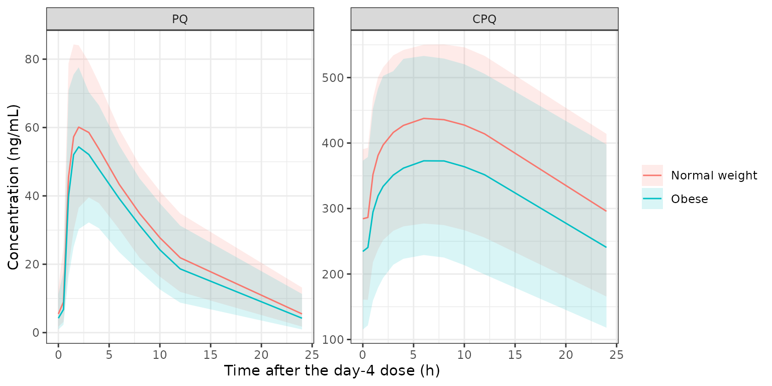
Simulated day-4 plasma PQ and CPQ after 15 mg once daily (individual predictions, median and 5th-95th percentiles, 200 virtual men per arm). Compare with the VPCs of Lee 2021 Figure 4B and 4C.
As in Figure 4, concentrations of both analytes are lower in the obese arm.
PKNCA validation
PKNCA computes the day-14 dosing-interval AUC (the Table 3 endpoint)
and the day-4 Cmax and Tmax per subject. It uses the individual
predictions Cc and Cc_cpq, which carry
between-subject variability but no residual error, as an AUC-based
summary such as Table 3 does.
nca_input <- sim |>
  select(id, arm, time, PQ = Cc, CPQ = Cc_cpq) |>
  pivot_longer(c(PQ, CPQ), names_to = "analyte", values_to = "conc") |>
  filter(!is.na(conc))

dose_df <- ev |>
  filter(evid == 1) |>
  select(id, arm, time, amt) |>
  tidyr::crossing(analyte = c("PQ", "CPQ"))

conc_obj <- PKNCA::PKNCAconc(nca_input, conc ~ time | arm + analyte + id,
  concu = "ng/mL", timeu = "h")
dose_obj <- PKNCA::PKNCAdose(dose_df, amt ~ time | arm + analyte + id,
  doseu = "mg")
intervals <- data.frame(
  start = c(72, 312),
  end = c(96, 336),
  cmax = c(TRUE, FALSE),
  tmax = c(TRUE, FALSE),
  auclast = c(FALSE, TRUE)
)
nca_res <- PKNCA::pk.nca(PKNCA::PKNCAdata(conc_obj, dose_obj, intervals = intervals))
nca_tab <- as.data.frame(nca_res$result)

nca_summary <- nca_tab |>
  filter(PPTESTCD %in% c("cmax", "tmax", "auclast")) |>
  group_by(analyte, arm, PPTESTCD) |>
  summarise(mean = mean(PPORRES), sd = sd(PPORRES), median = median(PPORRES), .groups = "drop")
knitr::kable(nca_summary |>
  dplyr::rename("Analyte" = analyte, "Arm" = arm, "Parameter" = PPTESTCD,
                "Mean" = mean, "SD" = sd, "Median" = median),
  digits = 1,
caption = "Simulated NCA: day-4 Cmax/Tmax and day-14 AUCtau (ng*h/mL), 200 virtual men per arm.")| Analyte | Arm | Parameter | Mean | SD | Median |
|---|---|---|---|---|---|
| CPQ | Normal weight | auclast | 9344.4 | 2262.4 | 9508.1 |
| CPQ | Normal weight | cmax | 427.7 | 88.4 | 438.0 |
| CPQ | Normal weight | tmax | 6.4 | 1.2 | 6.0 |
| CPQ | Obese | auclast | 8063.2 | 2387.3 | 7982.7 |
| CPQ | Obese | cmax | 375.4 | 96.5 | 374.4 |
| CPQ | Obese | tmax | 6.1 | 1.4 | 6.0 |
| PQ | Normal weight | auclast | 638.2 | 157.9 | 619.5 |
| PQ | Normal weight | cmax | 62.8 | 13.8 | 61.7 |
| PQ | Normal weight | tmax | 2.3 | 1.0 | 2.0 |
| PQ | Obese | auclast | 544.9 | 151.2 | 550.2 |
| PQ | Obese | cmax | 56.5 | 13.1 | 55.8 |
| PQ | Obese | tmax | 2.4 | 1.0 | 2.0 |
Comparison against Table 3
Table 3 reports the simulated steady-state AUCtau (mean +/- SD) after 15 mg daily for 14 days. Because Table 3 summarises by the mean, the simulated values below are aggregated to the arm mean before comparison.
published <- tibble::tribble(
  ~analyte, ~arm,            ~auclast,
  "PQ",     "Normal weight",   610.2,
  "PQ",     "Obese",           538.6,
  "CPQ",    "Normal weight",  8917,
  "CPQ",    "Obese",          7903.9
)
simulated <- nca_summary |>
  filter(PPTESTCD == "auclast") |>
  transmute(analyte, arm, PPTESTCD, PPORRES = mean)
cmp <- nlmixr2lib::ncaComparisonTable(
  simulated = simulated,
  reference = published,
  by = c("analyte", "arm"),
  units = c(auclast = "ng*h/mL"),
  tolerance_pct = 20
)
knitr::kable(cmp, caption = "Simulated arm-mean day-14 AUCtau vs Lee 2021 Table 3.")| NCA parameter | analyte | arm | Reference | Simulated | % diff |
|---|---|---|---|---|---|
| AUClast (ng*h/mL) | PQ | Normal weight | 610 | 638 | +4.6% |
| AUClast (ng*h/mL) | PQ | Obese | 539 | 545 | +1.2% |
| AUClast (ng*h/mL) | CPQ | Normal weight | 8920 | 9340 | +4.8% |
| AUClast (ng*h/mL) | CPQ | Obese | 7900 | 8060 | +2.0% |
# Weight-normalised AUC, the Table 3 rows marked '**'.
wn <- nca_tab |>
  filter(PPTESTCD == "auclast") |>
  left_join(cohort |> select(id, WT), by = "id") |>
  group_by(analyte, arm) |>
  summarise(auc_per_kg = mean(PPORRES / WT), .groups = "drop")
published_wn <- tibble::tribble(
  ~analyte, ~arm,            ~published,
  "PQ",     "Normal weight",   9.2,
  "PQ",     "Obese",           6.5,
  "CPQ",    "Normal weight", 134,
  "CPQ",    "Obese",          95.9
)
knitr::kable(wn |>
  left_join(published_wn, by = c("analyte", "arm")) |>
  dplyr::rename("Analyte" = analyte, "Arm" = arm,
                "Simulated AUCtau/WT" = auc_per_kg, "Table 3" = published),
digits = 1)| Analyte | Arm | Simulated AUCtau/WT | Table 3 |
|---|---|---|---|
| CPQ | Normal weight | 140.8 | 134.0 |
| CPQ | Obese | 98.5 | 95.9 |
| PQ | Normal weight | 9.7 | 9.2 |
| PQ | Obese | 6.7 | 6.5 |
auc_arm <- nca_tab |>
  filter(PPTESTCD == "auclast") |>
  group_by(analyte, arm) |>
  summarise(mean = mean(PPORRES), .groups = "drop") |>
  left_join(published, by = c("analyte", "arm"))
obese_ratio <- auc_arm |>
  group_by(analyte) |>
  summarise(ratio = mean[arm == "Obese"] / mean[arm == "Normal weight"], .groups = "drop")
# Arm means and the obese/normal contrast, not extremes; the per-arm mean of
# 200 subjects moves by a few percent between cohorts, a transcription error
# in a clearance or volume by tens of percent.
stopifnot(
  all(abs(auc_arm$mean / auc_arm$auclast - 1) < 0.15),
  all(obese_ratio$ratio < 1)
)
The simulated arm means sit close to Table 3 for both analytes and both arms, and the obese arm has the lower exposure, as published. The per-kilogram contrast (Table 3’s roughly 29% lower weight-normalised AUC in the obese group) is driven mostly by the weight denominator itself.
Replicating Figure 5
Figure 5 examines virtual men of 60-100 kg with activity score 1.5 and height 175 cm. Panel A gives the flat 15 mg dose, panel B the weight-normalised 0.25 mg/kg dose, and panel C varies the activity score at 17.5 mg and 70 kg. The typical-value AUCtau shown here is the centre of the paper’s boxes.
wts <- c(60, 70, 80, 90, 100)
scen <- bind_rows(
  tibble::tibble(panel = "A: 15 mg", x = wts, WT = wts, CYP2D6 = 1.5, dose = 15),
  tibble::tibble(panel = "B: 0.25 mg/kg", x = wts, WT = wts, CYP2D6 = 1.5, dose = 0.25 * wts),
  tibble::tibble(panel = "C: 17.5 mg, 70 kg", x = seq(0, 2.5, by = 0.5), WT = 70,
                 CYP2D6 = seq(0, 2.5, by = 0.5), dose = 17.5)
) |>
  mutate(id = row_number(), HT = 175)
ev5 <- bind_rows(lapply(seq_len(nrow(scen)), function(i) {
  make_events(scen$id[i], scen$dose[i], 14, seq(312, 336, by = 0.05))
})) |>
  left_join(scen |> select(id, WT, HT, CYP2D6), by = "id")
sim5 <- as.data.frame(rxode2::rxSolve(mod_typ, ev5, returnType = "data.frame"))
#> ℹ omega/sigma items treated as zero: 'etalvc', 'etalclint_mao', 'etalclint_cyp2d6', 'etalka', 'etalcl_cpq', 'etaltlag'
#> Warning: multi-subject simulation without without 'omega'
fig5 <- sim5 |>
  group_by(id) |>
  summarise(auc = trap(time, Cc), .groups = "drop") |>
  left_join(scen, by = "id")
ggplot(fig5, aes(x, auc)) +
  geom_point() +
  geom_line() +
  facet_wrap(~panel, scales = "free_x") +
  expand_limits(y = 0) +
  labs(x = "Body weight (kg) [A, B] or CYP2D6 activity score [C]",
       y = "PQ AUCtau (ng*h/mL)") +
  theme_bw()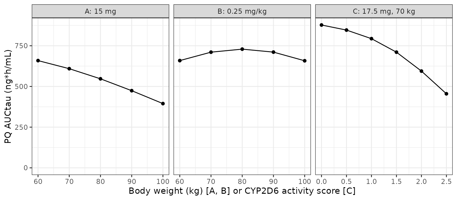
Typical-value steady-state PQ AUCtau: (A) 15 mg flat and (B) 0.25 mg/kg by body weight; (C) by CYP2D6 activity score at 17.5 mg, 70 kg. Replicates the centres of Lee 2021 Figure 5.
a <- fig5 |> filter(panel == "A: 15 mg") |> arrange(WT)
b <- fig5 |> filter(panel == "B: 0.25 mg/kg") |> arrange(WT)
c5 <- fig5 |> filter(panel == "C: 17.5 mg, 70 kg") |> arrange(CYP2D6)
per10kg <- 100 * (1 - (a$auc[5] / a$auc[1])^(1 / 4))
knitr::kable(tibble::tibble(
  Statement = c("AUC at 100 kg vs 60 kg, 15 mg (Discussion: ~40% smaller)",
                "Mean decrease per 10 kg, 15 mg (Results: ~12%)",
                "Max/min AUC across 60-100 kg at 0.25 mg/kg (Results: similar)"),
  Model = c(100 * (1 - a$auc[5] / a$auc[1]), per10kg, max(b$auc) / min(b$auc))
), digits = 2)| Statement | Model |
|---|---|
| AUC at 100 kg vs 60 kg, 15 mg (Discussion: ~40% smaller) | 40.09 |
| Mean decrease per 10 kg, 15 mg (Results: ~12%) | 12.02 |
| Max/min AUC across 60-100 kg at 0.25 mg/kg (Results: similar) | 1.11 |
stopifnot(
  abs(100 * (1 - a$auc[5] / a$auc[1]) - 40) < 5,
  abs(per10kg - 12) < 3,
  # 0.25 mg/kg: typical AUC peaks mid-range (80 kg) and is ~11% above the
  # 60 / 100 kg ends; the paper calls this 'similar'.
  max(b$auc) / min(b$auc) < 1.15,
  all(diff(c5$auc) < 0)
)
The flat dose loses about 40% of exposure between 60 and 100 kg, and the weight-normalised dose holds the typical AUC within about 11% across the whole range (highest at 80 kg, equal at 60 and 100 kg), as the Results and Discussion describe. Panel C declines monotonically with activity score.
Assumptions and deviations
-
Hepatic extraction ratio. Lee 2021 uses EH in
Figure 2B without defining it. The packaged model uses the well-stirred
definition of Goncalves 2017, the model Lee 2021 states it built on; the
Table 3 check above excludes the alternative literal reading. Using
CL_intdirectly as the liver-to-sink rate withEH = 0would give identical steady-state AUCs and differs only in the liver residence time, which is on the order of a minute. -
IIV scale. Table 2 reports each BSV as “CV%”. Its
RSE column cannot be on the variance scale (two rows fall below the
sqrt(2/24)= 28.9% floor for a variance from 24 subjects), so the CV% is read as100 * omegaand the variance entered as(CV/100)^2. Reading it as a log-normal CV,log(1 + CV^2), changes the KA variance most (0.687 vs 0.523), the CL_CYP variance by 13% and the others by under 3%; none of the AUC checks above depend on KA. The simulated between-subject SDs of AUCtau in the Table 3 comparison come out close to the published SDs (Table 3: PQ 149.5 and 160.2 ngh/mL; CPQ 2323.4 and 2521.9 ngh/mL), which is consistent with this reading. - Residual error. Equation (2) is a combined proportional + additive model, but Table 2 lists only a proportional term for PQ, so PQ carries proportional error only and CPQ both terms.
- Covariate coefficients. The Table 2 values (1.254, 0.041) are used rather than the rounded coefficients (1.25, 0.04) printed in the Section 3.2.2 equation. The CL_CYP centring weight 77.45 kg is from that equation.
- Mass units. PQ is converted to CPQ mass-for-mass, as the authors did (Section 2.5.2: molar conversion was not applied because the molecular weights, 259.35 and 274.31 g/mol, are close). Doses are in mg and concentrations in ng/mL.
- Hydroxychloroquine. The study co-administered hydroxychloroquine on days 1-3; the model has no term for it and the paper does not estimate one.
- Activity-score range. The study had activity scores 0.5-2.0 only. Figure 5C and this vignette extrapolate the exponential covariate model to 0 and 2.5 as the paper does.
- Virtual cohort. Weight and height are drawn from normal distributions matching the Table 1 group means and SDs and the activity score from each group’s Table 1 counts; the paper does not describe the covariates of its Table 3 simulation.