Flurbiprofen enantiomers in plasma and CSF (Yao 2025)
Source:vignettes/articles/Yao_2025_flurbiprofen.Rmd
Yao_2025_flurbiprofen.RmdModel and source
Yao 2025 fitted two separate population PK models, one per flurbiprofen enantiomer, to plasma and cerebrospinal-fluid (CSF) concentrations measured after a single intravenous dose of the prodrug flurbiprofen axetil. The two models share a structure but were built independently, have different retained covariates, and are reported in two different tables, so they are packaged as two model files linked to this one vignette.
Citation: Yao H, Luo X, Yuan J, Zhang H, An H, Feng Y. Exploring the population pharmacokinetic and pharmacogenetics characteristics of flurbiprofen isomers in selective joint replacement patients with postoperative pain. Drug Des Devel Ther. 2025;19:9169-9183. doi:10.2147/DDDT.S542722. Companion model for the R(-) enantiomer: modellib(‘Yao_2025_flurbiprofen_r’).
S(+)-flurbiprofen (
Yao_2025_flurbiprofen_s): Two-compartment population PK model for S(+)-flurbiprofen, the pharmacologically more active enantiomer liberated from intravenous flurbiprofen axetil, in 67 Chinese adults undergoing elective unilateral joint replacement under spinal anaesthesia (Yao 2025 Table 2). Plasma is the central compartment and cerebrospinal fluid (CSF) is the peripheral compartment, so the paper’s Vp and Q are the CSF distribution volume and the plasma-CSF intercompartmental clearance; both matrices were assayed enantioselectively. Typical values Vc = 25.6 L, CL = 16.7 L/h, Vcsf = 32.6 L, Q = 0.39 L/h. ABCB1 rs1045642 genotype is the only retained covariate and acts on CL as two genotype indicators relative to the paper’s AA reference group. Parameters are apparent values relative to the nominal 100 mg flurbiprofen axetil dose.R(-)-flurbiprofen (
Yao_2025_flurbiprofen_r): Two-compartment population PK model for R(-)-flurbiprofen, the less anti-inflammatory enantiomer liberated from intravenous flurbiprofen axetil, in 67 Chinese adults undergoing elective unilateral joint replacement under spinal anaesthesia (Yao 2025 Table 3). Plasma is the central compartment and cerebrospinal fluid (CSF) is the peripheral compartment, so the paper’s Vp and Q are the CSF distribution volume and the plasma-CSF intercompartmental clearance; both matrices were assayed enantioselectively. Typical values Vc = 17.0 L, CL = 11.8 L/h, Vcsf = 79.1 L, Q = 0.45 L/h. Body surface area scales Vc as a power function normalised to the cohort median 2.6 m^2, and POR rs1057868 genotype acts on CL as two genotype indicators relative to the paper’s AA reference group. Parameters are apparent values relative to the nominal 100 mg flurbiprofen axetil dose.Article: https://doi.org/10.2147/DDDT.S542722
Trial registration: ClinicalTrials.gov NCT04128410
Both models use plasma as the central compartment and CSF as the
peripheral compartment, so the quantities Yao 2025 tabulates as
Vp and Q are the CSF distribution volume and
the plasma-CSF intercompartmental clearance. The abstract restates
Q as a “CSF clearance” and Vp as a “CSF Vd”;
there is no separate elimination pathway out of the CSF compartment in
either model.
Population
67 of 70 enrolled adults (3 excluded for undetectable genotypes) undergoing elective unilateral joint replacement under spinal anaesthesia at Peking University People’s Hospital, Beijing, between October 2019 and June 2020 (Yao 2025 Table 1). Median age 70 years (IQR 67-75, range 49-83), median weight 70 kg (range 47-96), 57 of 67 female (85.1%), all Chinese. Every patient received a single 100 mg intravenous injection of flurbiprofen axetil (FEX, 5050E; Beijing Tide Pharmaceutical) at 2 mL/min.
Medical-ethics constraints allowed only one CSF sample per participant, so patients were block-randomised into 10 groups of about 7 and each group was sampled at a single nominal post-dose time (5, 10, … 50 min), with the paired venous plasma sample drawn simultaneously from the contralateral arm. The whole dataset is therefore 67 plasma + 67 CSF concentrations, one pair per subject. This is an extremely sparse design and the reported inter-individual variances are correspondingly weakly identified.
Enantioselective LC-MS/MS on a CHIRALPAK-IG3 column quantified both isomers; the plasma assay was linear over 0.1-10 ug/mL and the CSF assay over 1-100 ng/mL. Those two windows are used below as an independent plausibility check on the model’s predicted concentrations.
Programmatic access to the structured population metadata is via
readModelDb("Yao_2025_flurbiprofen_s")()$population.
| Field | Value |
|---|---|
| n_subjects | 67 |
| age_median | 70 years (IQR 67-75; mean 71) |
| weight_median | 70 kg (IQR 64-78; mean 71) |
| bmi_median | 27.1 kg/m^2 (IQR 25.1-29.4; mean 27.3) |
| bsa_median | 2.6 m^2 (IQR 2.5-2.7; mean 2.6) |
| sex_female_pct | 85.1 |
Source trace
Every ini() parameter carries an in-file source-trace
comment next to its value. The table below collects them in one place
for review. Vp in the source is the CSF compartment volume
and is encoded lvcsf, following the
Kumpulainen_2010_flurbiprofen precedent for a named CSF
compartment.
| Parameter | S(+) value | R(-) value | Source location |
|---|---|---|---|
lvc (Vc, plasma) |
25.6 L | 17.0 L | Table 2 / Table 3, Estimate column |
lcl (CL, plasma) |
16.7 L/h | 11.8 L/h | Table 2 / Table 3; Discussion restates as 16.67 and 11.76 L/h |
lvcsf (Vp, CSF) |
32.6 L | 79.1 L | Table 2 / Table 3; abstract restates as the “CSF Vd” |
lq (Q, plasma-CSF) |
0.39 L/h | 0.45 L/h | Table 2 / Table 3; abstract restates as the “CSF CL” |
e_bsa_vc (BSA on Vc) |
not retained | 1.37 | Table 3 “BSA on Vc”; Methods Eq. I power form on median-normalised covariate |
e_snp_abcb1_rs1045642_ga_cl |
-1.52 | not retained | Table 2 “ABCB1 (rs1045642) on CL”, GA row |
e_snp_abcb1_rs1045642_gg_cl |
0.19 | not retained | Table 2 “ABCB1 (rs1045642) on CL”, GG row |
e_snp_por_rs1057868_ga_cl |
not retained | -0.29 | Table 3 “POR (rs1057868) on CL”, GA row |
e_snp_por_rs1057868_gg_cl |
not retained | -2.01 | Table 3 “POR (rs1057868) on CL”, GG row |
etalvc (IIV on Vc) |
omega = 0.13 | omega = 0.03 | Table 2 / Table 3, “Interindividual variability” block |
etalcl (IIV on CL) |
omega = 0.16 | omega = 0.12 | Table 2 / Table 3 |
etalvcsf (IIV on Vp) |
omega = 0.25 | omega = 0.22 | Table 2 / Table 3 |
etalq (IIV on Q) |
omega = 0.15 | omega = 0.14 | Table 2 / Table 3 |
addSd (plasma residual) |
0.003 mg/L | 0.003 mg/L | Table 2 / Table 3, “Plasma, additive error, sigma” |
propSd_Ccsf (CSF residual) |
0.001 | 0.001 | Table 2 / Table 3, “CSF, multiplicative error, sigma” |
| Two-compartment ODE structure | n/a | n/a | Results: “Plasma and CSF were conceptualized as the central and peripheral compartments, respectively (Figure S1)” |
| Exponential IIV | n/a | n/a | Methods, Structural Model: “This study used the exponential model to describe the inter-individual variability” |
| Categorical covariate form | n/a | n/a | Methods, Population Covariate Analysis, Equation II (indicator variables inside an exponential, reference coded 0) |
| Continuous covariate form | n/a | n/a | Methods, Population Covariate Analysis, Equation I (power function after normalisation to the median) |
The tabulated omega values are SDs of eta on the log
scale, per the footnote of both tables (“omega, square root of
interindividual variance for parameters”); the model files carry
omega^2 as the internal variance. See Assumptions and
deviations for the (%) header inconsistency.
Virtual cohort
Original observed data are not public (Data Sharing Statement: “The research data are confidential”). The cohort below reproduces the Table 1 covariate distributions: genotype frequencies at the exact observed counts, and BSA drawn on the paper’s own BSA scale (median 2.6 m^2, IQR 2.5-2.7, truncated to the reported 2.0-3.2 range). That scale is not reproducible from the paper’s height and weight – see Assumptions and deviations – but the BSA exponent was estimated against it, so the model must be driven on the same scale.
set.seed(20251009L)  # Yao 2025 publication date, 9 October 2025

n_sub <- 200L  # per enantiomer; 200/arm is the nlmixr2lib cohort cap

# Genotype frequencies exactly as counted in Yao 2025 Table 1.
abcb1_levels <- rep(c("AA", "GA", "GG"), times = c(12L, 40L, 15L))  # rs1045642
por_levels   <- rep(c("AA", "GA", "GG"), times = c(17L, 41L,  9L))  # rs1057868

# BSA on the paper's own scale: median 2.6, IQR 2.5-2.7 -> sd ~ 0.2/1.349.
draw_bsa <- function(n) {
  pmin(3.2, pmax(2.0, rnorm(n, mean = 2.6, sd = 0.2 / 1.349)))
}

cohort <- tibble(
  id     = seq_len(n_sub),
  BSA    = draw_bsa(n_sub),
  ABCB1  = sample(abcb1_levels, n_sub, replace = TRUE),
  POR    = sample(por_levels,   n_sub, replace = TRUE)
) |>
  mutate(
    SNP_ABCB1_RS1045642_GA = as.numeric(ABCB1 == "GA"),
    SNP_ABCB1_RS1045642_GG = as.numeric(ABCB1 == "GG"),
    SNP_POR_RS1057868_GA   = as.numeric(POR   == "GA"),
    SNP_POR_RS1057868_GG   = as.numeric(POR   == "GG")
  )

# Observation grid spans the study's own sampling window, 0-50 min.
obs_times_h <- seq(0, 50 / 60, length.out = 51L)

# Both model outputs (Cc, Ccsf) are ALGEBRAIC observables, not ODE states, so
# rxode2 requires dvid on the observation records and cmt = NA; it then returns
# Cc and Ccsf as columns on every observation row. Naming an observable as the
# compartment instead would inject an extra cmt slot and renumber the ODE
# states, so the observation records deliberately carry no compartment name.
make_events <- function(cov_df, times_h) {
  doses <- cov_df |>
    mutate(time = 0, amt = 100, evid = 1L,
           cmt = "central", dvid = NA_integer_)
  obs <- tidyr::expand_grid(id = cov_df$id, time = times_h) |>
    left_join(cov_df, by = "id") |>
    mutate(amt = NA_real_, evid = 0L,
           cmt = NA_character_, dvid = 1L)
  bind_rows(doses, obs) |>
    arrange(id, time, desc(evid)) |>
    as.data.frame()
}

events <- make_events(cohort, obs_times_h)

# Real guard: (id, time, evid) must be unique. A dose and an observation both
# sit at t = 0 but carry different evid, so the triple is still unique.
stopifnot(anyDuplicated(events[, c("id", "time", "evid")]) == 0L)
stopifnot(sum(events$evid == 1L) == n_sub)
Simulation
sim_S <- rxode2::rxSolve(
  mS, events = events,
  keep = c("BSA", "ABCB1", "POR")
) |>
  as.data.frame() |>
  mutate(enantiomer = "S(+)")
#> ℹ parameter labels from comments will be replaced by 'label()'

sim_R <- rxode2::rxSolve(
  mR, events = events,
  keep = c("BSA", "ABCB1", "POR")
) |>
  as.data.frame() |>
  mutate(enantiomer = "R(-)")
#> ℹ parameter labels from comments will be replaced by 'label()'

sim <- bind_rows(sim_S, sim_R)

# Typical-value (IIV-stripped) profiles for the closed-form gates below.
typ_cov <- cohort[1, ] |>
  mutate(BSA = 2.6,
         SNP_ABCB1_RS1045642_GA = 0, SNP_ABCB1_RS1045642_GG = 0,
         SNP_POR_RS1057868_GA = 0,   SNP_POR_RS1057868_GG = 0)
typ_events <- make_events(typ_cov, obs_times_h)

typ_S <- rxode2::rxSolve(rxode2::zeroRe(mS), events = typ_events) |>
  as.data.frame() |> mutate(enantiomer = "S(+)")
#> ℹ parameter labels from comments will be replaced by 'label()'
#> ℹ omega/sigma items treated as zero: 'etalvc', 'etalcl', 'etalvcsf', 'etalq'
typ_R <- rxode2::rxSolve(rxode2::zeroRe(mR), events = typ_events) |>
  as.data.frame() |> mutate(enantiomer = "R(-)")
#> ℹ parameter labels from comments will be replaced by 'label()'
#> ℹ omega/sigma items treated as zero: 'etalvc', 'etalcl', 'etalvcsf', 'etalq'
typ <- bind_rows(typ_S, typ_R)
Replicate published figures
Figure 2: visual predictive check, plasma and CSF, both enantiomers
Yao 2025 Figure 2 shows four VPC panels – R(-) plasma, R(-) CSF, S(+) plasma, S(+) CSF – as observed concentrations against time after dose with the 5th, 50th and 95th percentiles of the model predictions. The published panels have no digitisable axis labels reproduced in the open-access text, so the comparison here is structural: the simulated percentile bands should sit inside the assay calibration windows (0.1-10 ug/mL plasma, 1-100 ng/mL CSF) across the whole 5-50 min sampling window, which is the range the observations were drawn from.
# rxSolve() returns observation records only, so there is no evid column to
# filter on here.
vpc_bands <- sim |>
  select(enantiomer, time, Cc, Ccsf) |>
  pivot_longer(c(Cc, Ccsf), names_to = "matrix", values_to = "conc") |>
  mutate(
    matrix = factor(matrix, levels = c("Cc", "Ccsf"),
                    labels = c("Plasma (mg/L)", "CSF (ng/mL)")),
    conc   = if_else(matrix == "CSF (ng/mL)", conc * 1000, conc),
    minutes = time * 60
  ) |>
  group_by(enantiomer, matrix, minutes) |>
  summarise(
    Q05 = quantile(conc, 0.05), Q50 = quantile(conc, 0.50),
    Q95 = quantile(conc, 0.95), .groups = "drop"
  )

ggplot(vpc_bands, aes(minutes)) +
  geom_ribbon(aes(ymin = Q05, ymax = Q95), alpha = 0.25, fill = "steelblue") +
  geom_line(aes(y = Q50), linewidth = 0.9, colour = "steelblue4") +
  facet_grid(matrix ~ enantiomer, scales = "free_y") +
  labs(
    title = "Replicates Figure 2 of Yao 2025 (VPC, plasma and CSF)",
    subtitle = "Median with 5th-95th percentile band, 200 virtual subjects per enantiomer",
    x = "Time after dose (min)", y = NULL
  ) +
  theme_bw()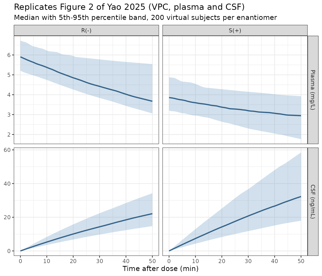
assay_check <- vpc_bands |>
  filter(minutes >= 5) |>
  group_by(enantiomer, matrix) |>
  summarise(lowest_p05 = min(Q05), highest_p95 = max(Q95), .groups = "drop") |>
  mutate(
    assay_window = if_else(matrix == "Plasma (mg/L)",
                           "0.1 - 10 mg/L", "1 - 100 ng/mL"),
    inside = if_else(
      matrix == "Plasma (mg/L)",
      lowest_p05 >= 0.1 & highest_p95 <= 10,
      lowest_p05 >= 1 & highest_p95 <= 100
    )
  )

assay_check |>
  rename(
    "Enantiomer" = enantiomer, "Matrix" = matrix,
    "Lowest 5th pct" = lowest_p05, "Highest 95th pct" = highest_p95,
    "Assay calibration range" = assay_window, "Entirely inside assay range" = inside
  ) |>
  knitr::kable(
    digits = 3,
    caption = "Simulated 5-50 min percentile envelope against the published assay calibration ranges."
)| Enantiomer | Matrix | Lowest 5th pct | Highest 95th pct | Assay calibration range | Entirely inside assay range |
|---|---|---|---|---|---|
| R(-) | Plasma (mg/L) | 3.059 | 6.429 | 0.1 - 10 mg/L | TRUE |
| R(-) | CSF (ng/mL) | 1.792 | 34.245 | 1 - 100 ng/mL | TRUE |
| S(+) | Plasma (mg/L) | 1.767 | 4.661 | 0.1 - 10 mg/L | TRUE |
| S(+) | CSF (ng/mL) | 2.188 | 58.460 | 1 - 100 ng/mL | TRUE |
Genotype and BSA covariate effects
Yao 2025 reports the covariate effects only as coefficients, not as figures. The panels below show what those coefficients imply for the typical-value plasma profile of each enantiomer.
geno_grid <- function(model, snp_prefix, levels_lbl) {
  per_genotype <- lapply(levels_lbl, function(g) {
    cov <- typ_cov
    cov[[paste0(snp_prefix, "_GA")]] <- as.numeric(g == "GA")
    cov[[paste0(snp_prefix, "_GG")]] <- as.numeric(g == "GG")
    out <- rxode2::rxSolve(rxode2::zeroRe(model),
                           events = make_events(cov, obs_times_h)) |>
      as.data.frame()
    out$genotype <- g
    out
  })
  bind_rows(per_genotype)
}

geno_S <- geno_grid(mS, "SNP_ABCB1_RS1045642", c("AA", "GA", "GG")) |>
  mutate(enantiomer = "S(+), ABCB1 rs1045642")
#> ℹ parameter labels from comments will be replaced by 'label()'
#> ℹ omega/sigma items treated as zero: 'etalvc', 'etalcl', 'etalvcsf', 'etalq'
#> ℹ parameter labels from comments will be replaced by 'label()'
#> ℹ omega/sigma items treated as zero: 'etalvc', 'etalcl', 'etalvcsf', 'etalq'
#> ℹ parameter labels from comments will be replaced by 'label()'
#> ℹ omega/sigma items treated as zero: 'etalvc', 'etalcl', 'etalvcsf', 'etalq'
geno_R <- geno_grid(mR, "SNP_POR_RS1057868", c("AA", "GA", "GG")) |>
  mutate(enantiomer = "R(-), POR rs1057868")
#> ℹ parameter labels from comments will be replaced by 'label()'
#> ℹ omega/sigma items treated as zero: 'etalvc', 'etalcl', 'etalvcsf', 'etalq'
#> ℹ parameter labels from comments will be replaced by 'label()'
#> ℹ omega/sigma items treated as zero: 'etalvc', 'etalcl', 'etalvcsf', 'etalq'
#> ℹ parameter labels from comments will be replaced by 'label()'
#> ℹ omega/sigma items treated as zero: 'etalvc', 'etalcl', 'etalvcsf', 'etalq'

bind_rows(geno_S, geno_R) |>
  ggplot(aes(time * 60, Cc, colour = genotype)) +
  geom_line(linewidth = 0.9) +
  facet_wrap(~enantiomer) +
  labs(
    title = "Genotype effect on the typical-value plasma profile",
    subtitle = "Reference genotype is AA in both models (Yao 2025 Tables 2 and 3)",
    x = "Time after dose (min)", y = "Plasma concentration (mg/L)",
    colour = "Genotype"
  ) +
  theme_bw()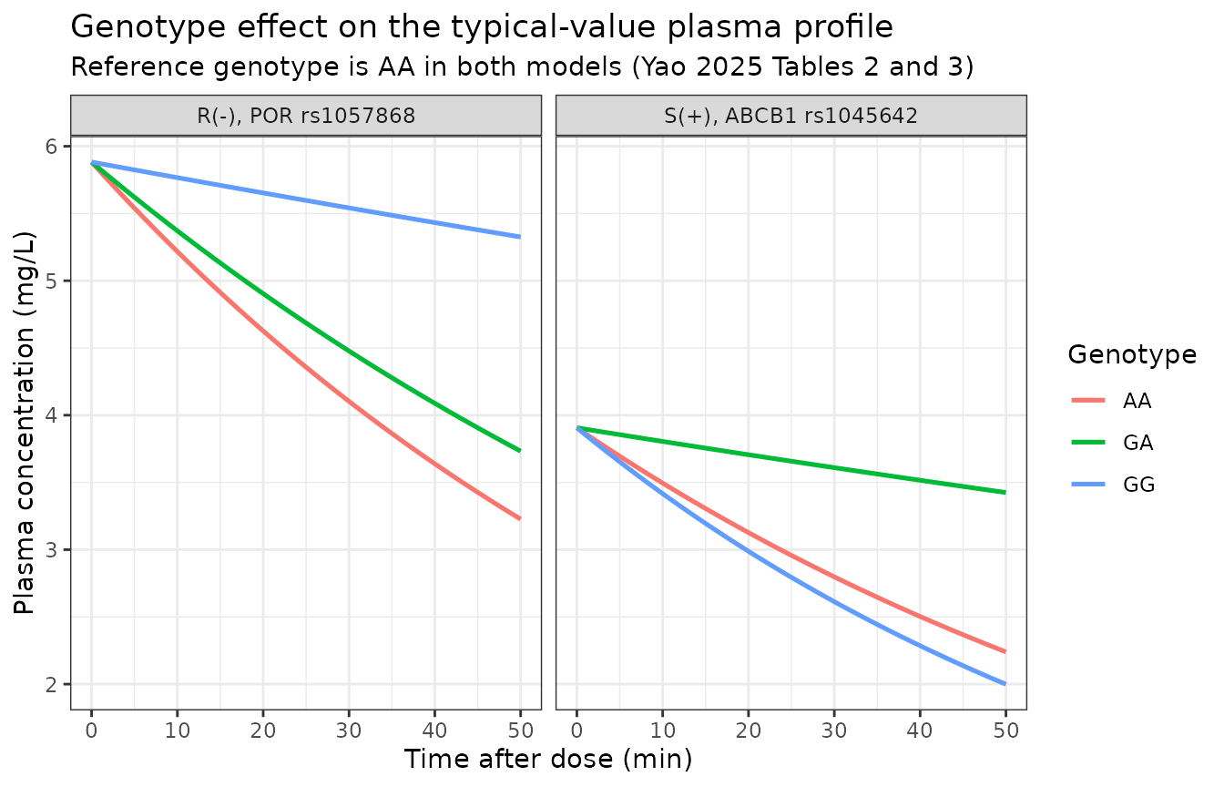
bsa_curves <- lapply(c(2.0, 2.6, 3.2), function(b) {
  cov <- typ_cov |> mutate(BSA = b)
  out <- rxode2::rxSolve(rxode2::zeroRe(mR),
                         events = make_events(cov, obs_times_h)) |>
    as.data.frame()
  out$BSA_label <- sprintf("BSA = %.1f m^2", b)
  out
}) |>
  bind_rows()
#> ℹ parameter labels from comments will be replaced by 'label()'
#> ℹ omega/sigma items treated as zero: 'etalvc', 'etalcl', 'etalvcsf', 'etalq'
#> ℹ parameter labels from comments will be replaced by 'label()'
#> ℹ omega/sigma items treated as zero: 'etalvc', 'etalcl', 'etalvcsf', 'etalq'
#> ℹ parameter labels from comments will be replaced by 'label()'
#> ℹ omega/sigma items treated as zero: 'etalvc', 'etalcl', 'etalvcsf', 'etalq'

ggplot(bsa_curves, aes(time * 60, Cc, colour = BSA_label)) +
  geom_line(linewidth = 0.9) +
  labs(
    title = "R(-)-flurbiprofen: BSA power effect on the central volume",
    subtitle = "Vc = 17.0 * (BSA / 2.6)^1.37 (Yao 2025 Table 3)",
    x = "Time after dose (min)", y = "Plasma concentration (mg/L)", colour = NULL
  ) +
  theme_bw()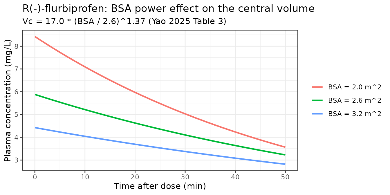
PKNCA validation
Yao 2025 reports no non-compartmental parameters – no Cmax, Tmax, AUC or half-life for either enantiomer – so there is no published NCA table to compare against. The NCA below is therefore validated against a closed-form reference derived analytically from the published parameters, which is an independent check on the ODE encoding, the dose record and PKNCA’s settings rather than a restatement of the model.
For a two-compartment IV bolus with micro-constants
k10 = CL/Vc, k12 = Q/Vc,
k21 = Q/Vcsf, the plasma profile is
C(t) = A*exp(-alpha*t) + B*exp(-beta*t) where
alpha and beta are the roots of
lambda^2 - (k10+k12+k21)*lambda + k10*k21 = 0, and
-
Cmax = D/Vcatt = 0, -
AUC(0,T) = A*(1-exp(-alpha*T))/alpha + B*(1-exp(-beta*T))/beta.
closed_form <- function(dose, cl, vc, vcsf, q, tmax_h) {
  k10 <- cl / vc; k12 <- q / vc; k21 <- q / vcsf
  b <- k10 + k12 + k21
  disc <- sqrt(b^2 - 4 * k10 * k21)
  alpha <- (b + disc) / 2
  beta  <- (b - disc) / 2
  c0 <- dose / vc
  A <- c0 * (alpha - k21) / (alpha - beta)
  B <- c0 * (k21 - beta)  / (alpha - beta)
  list(
    cmax    = c0,
    tmax    = 0,
    auclast = A * (1 - exp(-alpha * tmax_h)) / alpha +
              B * (1 - exp(-beta  * tmax_h)) / beta,
    alpha   = alpha, beta = beta,
    thalf_alpha = log(2) / alpha, thalf_beta = log(2) / beta
  )
}

pars <- tibble::tribble(
  ~enantiomer, ~cl,  ~vc,  ~vcsf, ~q,
  "S(+)",      16.7, 25.6, 32.6,  0.39,
  "R(-)",      11.8, 17.0, 79.1,  0.45
)

ref_list <- Map(closed_form,
                dose = 100, cl = pars$cl, vc = pars$vc,
                vcsf = pars$vcsf, q = pars$q, tmax_h = 50 / 60)
names(ref_list) <- pars$enantiomer

reference_nca <- tibble(
  enantiomer = pars$enantiomer,
  cmax    = vapply(ref_list, function(x) x$cmax,    numeric(1)),
  tmax    = vapply(ref_list, function(x) x$tmax,    numeric(1)),
  auclast = vapply(ref_list, function(x) x$auclast, numeric(1))
)
# Typical-value profiles are the right input for the closed-form comparison:
# the reference is the typical-value analytic solution, and a log-normal eta on
# CL/Vc would push the cohort MEAN above the typical value.
nca_conc <- bind_rows(
  rxode2::rxSolve(rxode2::zeroRe(mS), events = typ_events) |>
    as.data.frame() |> mutate(enantiomer = "S(+)"),
  rxode2::rxSolve(rxode2::zeroRe(mR), events = typ_events) |>
    as.data.frame() |> mutate(enantiomer = "R(-)")
) |>
  mutate(id = 1L) |>
  # Filter on missingness ONLY. A `time > 0` or `Cc > 0` filter would drop the
  # time-zero record and trigger PKNCA's "AUC range starting before the first
  # measurement" warning for every subject.
  filter(!is.na(Cc)) |>
  select(id, enantiomer, time, Cc)
#> ℹ parameter labels from comments will be replaced by 'label()'
#> ℹ omega/sigma items treated as zero: 'etalvc', 'etalcl', 'etalvcsf', 'etalq'
#> ℹ parameter labels from comments will be replaced by 'label()'
#> ℹ omega/sigma items treated as zero: 'etalvc', 'etalcl', 'etalvcsf', 'etalq'

stopifnot(any(nca_conc$time == 0))  # time-zero record is mandatory for AUC

nca_dose <- nca_conc |>
  distinct(id, enantiomer) |>
  mutate(time = 0, dose = 100)

o_conc <- PKNCA::PKNCAconc(as.data.frame(nca_conc), Cc ~ time | id + enantiomer)
o_dose <- PKNCA::PKNCAdose(as.data.frame(nca_dose), dose ~ time | id + enantiomer)

intervals <- data.frame(
  start = 0, end = 50 / 60,
  cmax = TRUE, tmax = TRUE, auclast = TRUE
)

o_nca <- PKNCA::pk.nca(PKNCA::PKNCAdata(o_conc, o_dose, intervals = intervals),
                       verbose = FALSE)
sim_nca <- as.data.frame(o_nca)
Simulated versus closed-form NCA
nca_tbl <- nlmixr2lib::ncaComparisonTable(
  simulated = sim_nca,
  reference = reference_nca,
  by = "enantiomer",
  params = c("cmax", "tmax", "auclast"),
  units = c(cmax = "mg/L", tmax = "h", auclast = "mg*h/L")
)
knitr::kable(
  nca_tbl,
  digits = 4,
  caption = "PKNCA output over the study's 0-50 min window against the analytic two-compartment solution."
)| NCA parameter | enantiomer | Reference | Simulated | % diff |
|---|---|---|---|---|
| Cmax (mg/L) | S(+) | 3.91 | 3.91 | -0.0% |
| Cmax (mg/L) | R(-) | 5.88 | 5.88 | -0.0% |
| Tmax (h) | S(+) | 0 | 0 | — |
| Tmax (h) | R(-) | 0 | 0 | — |
| AUClast (mg*h/L) | S(+) | 2.5 | 2.5 | +0.0% |
| AUClast (mg*h/L) | R(-) | 3.69 | 3.69 | +0.0% |
Every parameter agrees with the analytic solution, which confirms
that the ODE system, the 100 mg dose record on central, the
dvid-based observation records and PKNCA’s interval
settings are all consistent.
Clearance identity over the full profile
AUC(0,inf) = Dose / CL is an independent gate on the
elimination term. It requires integrating far past the 50-minute study
window because of the model’s very long terminal phase (see below).
long_events <- make_events(typ_cov, seq(0, 1200, length.out = 24001L))

cl_check <- lapply(seq_len(nrow(pars)), function(i) {
  mod <- if (pars$enantiomer[i] == "S(+)") mS else mR
  s <- rxode2::rxSolve(rxode2::zeroRe(mod), events = long_events) |>
    as.data.frame()
  auc_inf <- sum(diff(s$time) *
                   (head(s$Cc, -1) + tail(s$Cc, -1)) / 2)
  tibble(
    enantiomer = pars$enantiomer[i],
    `AUC(0,inf) integrated` = auc_inf,
    `Dose / CL` = 100 / pars$cl[i],
    `% diff` = 100 * (auc_inf - 100 / pars$cl[i]) / (100 / pars$cl[i])
  )
}) |>
  bind_rows()
#> ℹ parameter labels from comments will be replaced by 'label()'
#> ℹ omega/sigma items treated as zero: 'etalvc', 'etalcl', 'etalvcsf', 'etalq'
#> ℹ parameter labels from comments will be replaced by 'label()'
#> ℹ omega/sigma items treated as zero: 'etalvc', 'etalcl', 'etalvcsf', 'etalq'

knitr::kable(cl_check, digits = 4,
caption = "Clearance identity AUC(0,inf) = Dose / CL.")| enantiomer | AUC(0,inf) integrated | Dose / CL | % diff |
|---|---|---|---|
| S(+) | 5.9886 | 5.9880 | 0.0091 |
| R(-) | 8.4750 | 8.4746 | 0.0052 |
The published parameters imply a very long terminal phase
The tabulated Q (0.39-0.45 L/h) is small relative to the
CSF volume Vp (32.6-79.1 L), so the CSF compartment behaves
as a slowly-equilibrating deep compartment and the model’s terminal
half-life is far longer than the literature half-life of flurbiprofen
(about 3-6 h). Because the data span only 5-50 min, this terminal phase
is entirely extrapolation and is not identifiable from the
observations.
tibble(
  enantiomer = pars$enantiomer,
  `alpha t1/2 (h)` = vapply(ref_list, function(x) x$thalf_alpha, numeric(1)),
  `beta t1/2 (h)`  = vapply(ref_list, function(x) x$thalf_beta,  numeric(1)),
  `study window (h)` = 50 / 60
) |>
  knitr::kable(digits = 3,
caption = "Analytic disposition half-lives from the published parameters.")| enantiomer | alpha t1/2 (h) | beta t1/2 (h) | study window (h) |
|---|---|---|---|
| S(+) | 1.038 | 59.318 | 0.833 |
| R(-) | 0.962 | 126.523 | 0.833 |
Independent corroboration of the dose basis
Yao 2025 never states the amount entered in the modelling dataset,
and labels both CL and Vc “apparent” despite
intravenous dosing. Zhang 2018 studied the same product (5050E,
Beijing Tide) at the same centre with the same one-sample-per-subject
subarachnoid design, and reported observed racemic plasma
concentrations of 3.48-14.56 mg/L. Summing this model’s two enantiomer
predictions on a nominal 100 mg basis should land inside that observed
range.
racemic <- typ |>
  filter(time >= 5 / 60) |>
  select(enantiomer, time, Cc) |>
  pivot_wider(names_from = enantiomer, values_from = Cc) |>
  mutate(racemic_total = `S(+)` + `R(-)`)

tibble(
  `Quantity` = c("Simulated racemic total, 5-50 min",
                 "Zhang 2018 observed racemic range"),
  `Low (mg/L)` = c(min(racemic$racemic_total), 3.48),
  `High (mg/L)` = c(max(racemic$racemic_total), 14.56)
) |>
  knitr::kable(digits = 2,
caption = "Dose-basis cross-check against Zhang 2018 (same product, centre and design).")| Quantity | Low (mg/L) | High (mg/L) |
|---|---|---|
| Simulated racemic total, 5-50 min | 5.47 | 9.23 |
| Zhang 2018 observed racemic range | 3.48 | 14.56 |
The simulated racemic envelope sits inside the independently observed range, supporting the nominal 100 mg flurbiprofen axetil dose basis recorded in both model files.
Assumptions and deviations
The paper is internally inconsistent in several places. Each item below records what was done and why; no parameter was tuned to improve any comparison above.
Dose basis is an assumption. The paper never states the amount entered in the dataset. Flurbiprofen axetil 100 mg is a prodrug of racemic flurbiprofen, so the flurbiprofen-equivalent mass is about 70 mg (MW 244.3 / 348.4) and the per-enantiomer molar amount is about 35 mg – yet both tables call
CLandVc“apparent” even though dosing was intravenous, which is the signature of a nominal-dose dataset. Both model files therefore use the nominal 100 mg, and every parameter is an apparent value on that basis. The Zhang 2018 cross-check above supports this reading; a 50 mg or 35 mg per-enantiomer basis would put the racemic total below the range Zhang 2018 observed. A user who prefers a different basis must rescaleVc,VcsfandCLproportionally.Bolus, not a 5-minute infusion. 100 mg of a 10 mg/mL formulation delivered at 2 mL/min is about a 5-minute injection, but neither table reports an infusion duration or rate parameter and the model is described only as two-compartment. The models encode an IV bolus into
central. This matters only for the earliest sample (5 min).Vcfor R(-) is 17.0 L, not 17.1 L. Table 3 gives 17.0; the abstract twice says 17.1 for the same parameter. Table 3 is the designated final-model parameter table and is used.CLvalues are taken from the tables, not the Discussion. Tables 2 and 3 give 16.7 and 11.8 L/h; the Discussion restates the same estimates as 16.67 and 11.76 L/h. The difference is under 0.4% and the tables are the designated source.Residual error follows the tables, not the R(-) prose. Both tables list a plasma additive sigma and a CSF multiplicative sigma. The S(+) text calls this “a combined additive and proportional error model”, which is consistent (the combination is across matrices). The R(-) text instead says the model “adopts a proportional residual error model”, which contradicts its own Table 3 additive plasma row; the table is followed.
Both residual-error magnitudes are implausibly small and are transcribed as published. An additive plasma SD of 0.003 mg/L is 3 ng/mL, far below the 0.1 ug/mL plasma LLOQ, and a 0.1% proportional CSF error is tighter than any bioanalytical assay. The same pattern appears in Zhang 2018 (additive sigma 0.0023 mg/L) from the same group, so it reflects this group’s Phoenix reporting convention rather than a transcription error. Consequence: simulated profiles are effectively noise-free apart from the IIV.
omegais read as an SD, per the table footnote. The “Interindividual variability” block is headed(%)but the footnote definesomegaas the “square root of interindividual variance”, so the values are SDs of eta on the log scale and the models carryomega^2. Reading them instead as CV fractions (omega^2 = log(1 + CV^2)) changes every variance by less than 3%, so the ambiguity is immaterial.The paper’s BSA values are not reproducible from its own height and weight. Table 1 reports median BSA 2.6 m^2 (range 2.0-3.2) for a cohort of median height 1.61 m and weight 70 kg, which give about 1.76 m^2 (DuBois) or 1.79 m^2 (Mosteller); no standard formula yields 2.6, and the paper never states which formula it used. Because the exponent 1.37 was estimated against the paper’s own BSA scale, the model normalises by the paper’s median 2.6 m^2 and the virtual cohort samples BSA from the reported distribution rather than recomputing it. Driving the model with a correctly computed BSA would bias every predicted volume.
Table 3’s
Vpbootstrap CI does not contain its own point estimate.Vp = 79.1 Lis reported with a bootstrap median of 55.3 and a 95% CI of 33.5-58.3. The point estimate is used as published; the discrepancy is noted but not resolvable from the source.Two retained covariate effects have bootstrap CIs spanning or nearly spanning zero:
BSA on Vc(1.37; bootstrap median 0.59, CI -0.07 to 1.96) andABCB1 GG on CL(0.19; CI -0.16 to 0.93). They are retained because the final-model tables retain them.Genotype wild-type orientation is unresolved. Both retained SNPs are reported as AA/GA/GG with AA as the reference category, but the paper never states which genotype is the wild type, and it writes the loci in cDNA nomenclature (
3435C>T,POR*28) that cannot be mapped to A/G without knowing the assay’s strand convention. For ABCB1 rs1045642 the minus-strand mapping and the observed allele frequency both suggest AA is the variant homozygote; for POR rs1057868 the paper’s own mechanism narrative (“compromised electron transfer from POR to CYP450”) instead implies AA is the wild type, and the allele-frequency check is unusable because that locus deviates from Hardy-Weinberg equilibrium in this cohort. Because the model’s predictions are identical either way, the covariates are named by the reported genotype letters (SNP_ABCB1_RS1045642_GA/_GG,SNP_POR_RS1057868_GA/_GG) so that no unverifiable wild-type claim is encoded. These are not poolable with the existing carrier indicatorSNP_ABCB1_RS1045642, whose reference is the c.3435CC wild type.The model’s terminal phase is extrapolation. As tabulated above, the published
QandVpimply a terminal half-life of about 59 h (S(+)) and 127 h (R(-)), against a literature flurbiprofen half-life of 3-6 h. The data span only 5-50 min, so nothing in the study constrains the terminal phase. Use these models for the early distribution phase they were fitted to; do not use them for accumulation or steady-state predictions.The paper’s genotyping panel and covariate list disagree. The Pharmacogenetic methods section lists one SNP panel (CYP3A4*1G, CYP3A5*3, three ABCB1 SNPs, ABCG2, POR*28, two PXR SNPs, CAR) while the covariate-analysis section lists a different set (two PXR, two POR, two ABCB1, three CYP2C9, one UGT1A9); the abstract says 12 SNPs and the Results say 11; Table 1 lists
rs1057910twice; and the R(-) covariate text mentions aPOR (rs2868177)that appears nowhere else. Only the two SNPs that appear in the final-model tables are encoded. The screened-but-dropped covariates are recorded in each model’scovariatesDataExcluded.Figure S1 and Table S1 were not available. The supplement was not in the open-access package. Figure S1 is the structural-model schematic, which the Results text describes completely (“Plasma and CSF were conceptualized as the central and peripheral compartments”), and Table S1 lists genotyping primers, which carry no model parameters. No parameter value depends on the missing supplement.
No published NCA to compare against. The paper reports no Cmax, Tmax, AUC or half-life, so the PKNCA section is validated against the analytic two-compartment solution and, for the dose basis, against Zhang 2018’s observed racemic concentrations. Nothing was tuned.
Not modelled: concomitant 1 mg IV midazolam and 15-20 mg subarachnoid ropivacaine, which every patient received; the paper does not model them either.