Midazolam 24-hour variation (van Rongen 2015)
Source:vignettes/articles/vanRongen_2015_midazolam_circadian.Rmd
vanRongen_2015_midazolam_circadian.RmdModel and source
- Citation: van Rongen A, Kervezee L, Brill MJE, van Meir H, den Hartigh J, Guchelaar H-J, Meijer JH, Burggraaf J, van Oosterhout F (2015). Population Pharmacokinetic Model Characterizing 24-Hour Variation in the Pharmacokinetics of Oral and Intravenous Midazolam in Healthy Volunteers. CPT Pharmacometrics Syst Pharmacol 4(8):454-464. doi:10.1002/psp4.12007.
- Article: https://doi.org/10.1002/psp4.12007
- PubMed Central: https://www.ncbi.nlm.nih.gov/pmc/articles/PMC4562161/
mod <- rxode2::rxode2(readModelDb("vanRongen_2015_midazolam_circadian"))
#> ℹ parameter labels from comments will be replaced by 'label()'
#> Warning: some etas defaulted to non-mu referenced, possible parsing error: etaiov_fdepot_1, etaiov_fdepot_2, etaiov_fdepot_3, etaiov_fdepot_4, etaiov_fdepot_5, etaiov_fdepot_6
#> as a work-around try putting the mu-referenced expression on a simple line
van Rongen et al. gave 12 healthy volunteers a 2 mg oral midazolam solution followed 150 minutes later by a 1 mg intravenous bolus, and repeated that semi-simultaneous pair at six clock times spanning the 24-hour period. Because the oral and intravenous doses are given to the same subject within one profile, oral bioavailability, absorption rate and systemic clearance can be separated – which is what lets the paper attribute the observed daily rhythm to specific processes rather than to exposure as a whole.
Three chronopharmacologic terms came out of that analysis, and the packaged model carries all three:
- Oral bioavailability follows a 24-hour cosine about a mesor of 0.277, amplitude 0.041, peaking at 12:14.
- Clearance follows a 24-hour cosine about a mesor of 0.379 L/min, amplitude 0.027 L/min, peaking at 18:50.
- The absorption rate constant is multiplied by 1.41 when the oral dose is given at 14:00 – a step effect at one administration time, not a periodic function.
Population
pop <- readModelDb("vanRongen_2015_midazolam_circadian")()$population
#> Warning: some etas defaulted to non-mu referenced, possible parsing error: etaiov_fdepot_1, etaiov_fdepot_2, etaiov_fdepot_3, etaiov_fdepot_4, etaiov_fdepot_5, etaiov_fdepot_6
#> as a work-around try putting the mu-referenced expression on a simple line
tibble::tibble(Field = names(pop), Value = vapply(pop, as.character, character(1))) |>
knitr::kable(caption = "Population metadata (van Rongen 2015 Table 1 and Methods).")| Field | Value |
|---|---|
| species | human |
| n_subjects | 12 |
| n_studies | 1 |
| age_range | 18-27 years |
| age_median | 22 years (mean 21.8, SD 3.19) |
| weight_range | 63.4-92.9 kg |
| weight_median | 75.4 kg (mean 76.0, SD 8.65) |
| sex_female_pct | 0 |
| race_ethnicity | Caucasian (100 percent by inclusion criterion) |
| disease_state | Healthy, nonsmoking Caucasian male volunteers with body mass index 18-30 kg/m^2 (observed 18.8-25.8, median 21.9). Excluded for any clinically significant abnormality in medical history, routine laboratory tests or 12-lead ECG, for any medication use, for extreme morning or evening chronotype on the Horne-Ostberg questionnaire, and for transmeridian flights or shift work in the month before the study. |
| dose_range | Semi-simultaneous administration of 2 mg oral midazolam solution followed 150 minutes later by 1 mg intravenous midazolam, given twice per study visit at a 12-hour interval across three visits, so that oral administration occurred at 10:00, 14:00, 18:00, 22:00, 02:00 and 06:00. Washout at least 2 weeks between visits. Serum samples at 0, 15, 30, 45, 58, 65, 70, 75, 80, 90, 120, 148, 155, 165, 180, 210, 240, 270, 330 and 390 min after the oral dose, plus 715 min on the first half of a visit. Assay LLQ 0.3 ug/L. |
| regions | The Netherlands (Centre for Human Drug Research, Leiden) |
| notes | Demographics from Table 1 of van Rongen 2015 (n = 12). One subject withdrew consent during the study for personal reasons and was replaced by another subject dosed on the same randomization order, so 13 individuals were enrolled and 12 complete datasets were analyzed. Circadian entrainment was controlled and verified: subjects held a stable sleep-wake schedule for a week before each visit, wore an actigraph, remained semirecumbent, slept under dimmed lights with an eye mask from 23:30 to 07:30, and the expected 24-hour rhythms in serum TSH (29 percent relative amplitude, peak 03:05), heart rate (10 percent) and diastolic / systolic blood pressure (6.3 / 5.6 percent, peaks near 16:00) were confirmed by cosinor analysis as external validators. |
Twelve healthy, nonsmoking Caucasian men aged 18-27 years (median 22,
mean 21.8, SD 3.19) and weighing 63.4-92.9 kg (median 75.4) were studied
at the Centre for Human Drug Research in Leiden. Circadian entrainment
was actively controlled – a stable sleep-wake schedule for a week before
each visit, actigraphy, a semirecumbent posture throughout, and dimmed
lights with an eye mask from 23:30 to 07:30 – and verified through
external markers: serum TSH, heart rate and blood pressure all showed
the expected 24-hour rhythms on cosinor analysis. That control is what
makes the PK rhythm interpretable, so it is recorded in the model’s
population$notes.
Source trace
Every value in ini() comes from Table 2 of van Rongen
2015 (page 460), “Model estimates (RSE%)” column. The bootstrap column
of the same table (250/250 successful resamples) brackets every point
estimate.
tibble::tribble(
  ~Quantity, ~Parameter, ~Value, ~Source,
  "Clearance mesor",             "lcl",              "0.379 L/min (RSE 4.8%)",  "Table 2, row 'CLmesor (L/min)'",
  "Clearance cosine amplitude",  "amp_cl",           "0.027 L/min (RSE 14.8%)", "Table 2, row 'Amp (L/min)'",
  "Clearance cosine acrophase",  "acrophase_cl",     "1,130 min (RSE 2.9%)",    "Table 2, row 'Acrophase (min)' under CL",
  "Central volume",              "lvc",              "18.2 L (RSE 5.4%)",       "Table 2, row 'Vcentral (L)'",
  "Peripheral volumes (equal)",  "lvp",              "22.5 L (RSE 2.5%)",       "Table 2, row 'Vperipheral1 = Vperipheral2 (L)'",
  "Inter-compartmental CL Q",    "lq",               "0.27 L/min (RSE 6.8%)",   "Table 2, row 'Q (L/min)'",
  "Inter-compartmental CL Q2",   "lq2",              "1.31 L/min (RSE 8.5%)",   "Table 2, row 'Q2 (L/min)'",
  "Absorption = transit rate",   "lka",              "0.053 1/min (RSE 5.8%)",  "Table 2, row 'Ka = Ktr (min-1)'",
  "Ka factor at 14:00",          "e_tclock_ka",      "1.41 (RSE 4.7%)",         "Table 2, row 'Fraction Ka at 14:00'",
  "Bioavailability mesor",       "lfdepot",          "0.277 (RSE 7.1%)",        "Table 2, row 'F' under the F equation",
  "Bioavailability amplitude",   "amp_fdepot",       "0.041 (RSE 17.3%)",       "Table 2, row 'Amp' under the F equation",
  "Bioavailability acrophase",   "acrophase_fdepot", "734 min (RSE 5.3%)",      "Table 2, row 'Acrophase (min)' under F",
  "IIV clearance",               "etalcl",           "16.2% CV (RSE 21)",       "Table 2, interindividual variability, row 'CL (%)'",
  "IIV absorption rate",         "etalka",           "19.1% CV (RSE 21.9)",     "Table 2, interindividual variability, row 'Ka (%)'",
  "IIV bioavailability",         "etalfdepot",       "23.3% CV (RSE 22.2)",     "Table 2, interindividual variability, row 'F (%)'",
  "IOV bioavailability",         "etaiov_fdepot_1",  "14.8% CV (RSE 10.5)",     "Table 2, interoccasion variability, row 'F (%)'",
  "Residual error, oral",        "propSdOral",       "18.0% (RSE 5.6)",         "Table 2, residual proportional error, row 'sigma oral (%)'",
  "Residual error, intravenous", "propSdIv",         "15.4% (RSE 6.1)",         "Table 2, residual proportional error, row 'sigma intravenous (%)'"
) |>
knitr::kable(caption = "Source trace for every ini() value. Structural equations come from the Table 2 header rows (the two cosine equations) and from paper Equations 1-2.")| Quantity | Parameter | Value | Source |
|---|---|---|---|
| Clearance mesor | lcl | 0.379 L/min (RSE 4.8%) | Table 2, row ‘CLmesor (L/min)’ |
| Clearance cosine amplitude | amp_cl | 0.027 L/min (RSE 14.8%) | Table 2, row ‘Amp (L/min)’ |
| Clearance cosine acrophase | acrophase_cl | 1,130 min (RSE 2.9%) | Table 2, row ‘Acrophase (min)’ under CL |
| Central volume | lvc | 18.2 L (RSE 5.4%) | Table 2, row ‘Vcentral (L)’ |
| Peripheral volumes (equal) | lvp | 22.5 L (RSE 2.5%) | Table 2, row ‘Vperipheral1 = Vperipheral2 (L)’ |
| Inter-compartmental CL Q | lq | 0.27 L/min (RSE 6.8%) | Table 2, row ‘Q (L/min)’ |
| Inter-compartmental CL Q2 | lq2 | 1.31 L/min (RSE 8.5%) | Table 2, row ‘Q2 (L/min)’ |
| Absorption = transit rate | lka | 0.053 1/min (RSE 5.8%) | Table 2, row ‘Ka = Ktr (min-1)’ |
| Ka factor at 14:00 | e_tclock_ka | 1.41 (RSE 4.7%) | Table 2, row ‘Fraction Ka at 14:00’ |
| Bioavailability mesor | lfdepot | 0.277 (RSE 7.1%) | Table 2, row ‘F’ under the F equation |
| Bioavailability amplitude | amp_fdepot | 0.041 (RSE 17.3%) | Table 2, row ‘Amp’ under the F equation |
| Bioavailability acrophase | acrophase_fdepot | 734 min (RSE 5.3%) | Table 2, row ‘Acrophase (min)’ under F |
| IIV clearance | etalcl | 16.2% CV (RSE 21) | Table 2, interindividual variability, row ‘CL (%)’ |
| IIV absorption rate | etalka | 19.1% CV (RSE 21.9) | Table 2, interindividual variability, row ‘Ka (%)’ |
| IIV bioavailability | etalfdepot | 23.3% CV (RSE 22.2) | Table 2, interindividual variability, row ‘F (%)’ |
| IOV bioavailability | etaiov_fdepot_1 | 14.8% CV (RSE 10.5) | Table 2, interoccasion variability, row ‘F (%)’ |
| Residual error, oral | propSdOral | 18.0% (RSE 5.6) | Table 2, residual proportional error, row ‘sigma oral (%)’ |
| Residual error, intravenous | propSdIv | 15.4% (RSE 6.1) | Table 2, residual proportional error, row ‘sigma intravenous (%)’ |
The two cosine equations are printed verbatim as Table 2 header rows,
CL = CLmesor + Amp x cos((2*pi/1440)*(Time - Acrophase))
F  = Fmesor  + Amp x cos((2*pi/1440)*(Time - Acrophase))
with Time defined in the Methods as “the time in minutes
starting at midnight”. Paper Equation 1 places the random effects on the
population mean,
theta_ij = theta_mean * exp(eta_i + kappa_ij), and paper
Equation 2 defines the cosine’s first term as the individual
mesor – the value “around which it oscillates”. The random effects
therefore act on the mesor only and the amplitude carries none, which is
why the model adds the cosine component outside the exp()
rather than multiplying it.
Reproducing the paper’s chronopharmacologic summaries
The paper states its headline circadian quantities in Results, in the Discussion, and in the Figure 4 caption. Each is a deterministic function of the Table 2 values, so these are tight checks: a mis-transcribed amplitude, mesor or acrophase breaks them immediately.
hhmm <- function(min_after_midnight) {
  sprintf("%02d:%02d", min_after_midnight %/% 60, round(min_after_midnight %% 60))
}

# Printed Table 2 values, written out so this gate cannot be satisfied by
# reading the model back (a gate built from model variables cannot go red).
f_mesor  <- 0.277; f_amp  <- 0.041; f_acro  <- 734
cl_mesor <- 0.379; cl_amp <- 0.027; cl_acro <- 1130

chrono <- tibble::tribble(
  ~Quantity,                              ~Paper,   ~Reproduced,
  "F acrophase (clock time)",             "12:14",  hhmm(f_acro),
  "F relative amplitude (%)",             "14.7",   sprintf("%.1f", 100 * f_amp / f_mesor),
  "F peak-to-trough difference (%)",      "29.4",   sprintf("%.1f", 100 * 2 * f_amp / f_mesor),
  "CL acrophase (clock time)",            "18:50",  hhmm(cl_acro),
  "CL relative amplitude (%)",            "7.2",    sprintf("%.1f", 100 * cl_amp / cl_mesor),
  "CL peak-to-trough difference (%)",     "14.4",   sprintf("%.1f", 100 * 2 * cl_amp / cl_mesor)
)
knitr::kable(chrono, caption = "Paper-stated circadian summaries versus the values implied by Table 2. Sources: Results ('relative amplitude of 14.7% with a peak at 12:14' and '7.2% and a peak at 18:50'), Discussion ('relative difference between peak and trough values of 29.4%' and 'peak and trough levels of 14.4%'), and the Figure 4 caption.")| Quantity | Paper | Reproduced |
|---|---|---|
| F acrophase (clock time) | 12:14 | 12:14 |
| F relative amplitude (%) | 14.7 | 14.8 |
| F peak-to-trough difference (%) | 29.4 | 29.6 |
| CL acrophase (clock time) | 18:50 | 18:50 |
| CL relative amplitude (%) | 7.2 | 7.1 |
| CL peak-to-trough difference (%) | 14.4 | 14.2 |
stopifnot(
  hhmm(f_acro)  == "12:14",
  hhmm(cl_acro) == "18:50",
  abs(100 * f_amp  / f_mesor  - 14.7) < 0.2,
  abs(100 * cl_amp / cl_mesor -  7.2) < 0.2,
  abs(100 * 2 * f_amp  / f_mesor  - 29.4) < 0.3,
  abs(100 * 2 * cl_amp / cl_mesor - 14.4) < 0.3
)
The next check asks the packaged model the same question, by
solving a typical-value profile across a full day and locating the
clearance peak empirically. This exercises the clockTime
reconstruction and the cosine as written in model(), not
just the arithmetic above.
typical <- rxode2::zeroRe(mod)
#> Warning: No sigma parameters in the model
#> Warning: some etas defaulted to non-mu referenced, possible parsing error: etaiov_fdepot_1, etaiov_fdepot_2, etaiov_fdepot_3, etaiov_fdepot_4, etaiov_fdepot_5, etaiov_fdepot_6
#> as a work-around try putting the mu-referenced expression on a simple line

day <- data.frame(
  time = seq(0, 1439, by = 1),
  TCLOCK = 0, OCC = 1, ROUTE_IV = 0,
  evid = 0, amt = NA_real_, cmt = "central"
)
day_sol <- rxode2::rxSolve(typical, day, returnType = "data.frame")
#> ℹ omega/sigma items treated as zero: 'etalcl', 'etalka', 'etalfdepot', 'etaiov_fdepot_1', 'etaiov_fdepot_2', 'etaiov_fdepot_3', 'etaiov_fdepot_4', 'etaiov_fdepot_5', 'etaiov_fdepot_6'

emp_cl_acro <- day_sol$time[which.max(day_sol$cl)]
stopifnot(
  # TCLOCK = 0 anchors the solve at midnight, so model time is minutes after
  # midnight and the peak must land on the printed acrophase exactly.
  emp_cl_acro == cl_acro,
  abs(max(day_sol$cl) - (cl_mesor + cl_amp)) < 1e-6,
  abs(min(day_sol$cl) - (cl_mesor - cl_amp)) < 1e-6
)
sprintf("Model clearance peaks at %s (%.3f L/min) and troughs at %.3f L/min.",
        hhmm(emp_cl_acro), max(day_sol$cl), min(day_sol$cl))
#> [1] "Model clearance peaks at 18:50 (0.406 L/min) and troughs at 0.352 L/min."
The 14:00 absorption factor is a step effect, so it is checked at each of the six administration times the study used.
ka_at <- function(tclock) {
  d <- data.frame(time = 0:1, TCLOCK = tclock, OCC = 1, ROUTE_IV = 0,
                  evid = 0, amt = NA_real_, cmt = "central")
  rxode2::rxSolve(typical, d, returnType = "data.frame")$ka[1]
}
admin_times <- c(10, 14, 18, 22, 2, 6)
ka_tab <- tibble::tibble(
  `Administration time` = sprintf("%02d:00", admin_times),
  `Ka (1/min)` = vapply(admin_times, ka_at, numeric(1))
) |>
  mutate(`Factor vs 0.053` = `Ka (1/min)` / 0.053)
#> ℹ omega/sigma items treated as zero: 'etalcl', 'etalka', 'etalfdepot', 'etaiov_fdepot_1', 'etaiov_fdepot_2', 'etaiov_fdepot_3', 'etaiov_fdepot_4', 'etaiov_fdepot_5', 'etaiov_fdepot_6'
#> ℹ omega/sigma items treated as zero: 'etalcl', 'etalka', 'etalfdepot', 'etaiov_fdepot_1', 'etaiov_fdepot_2', 'etaiov_fdepot_3', 'etaiov_fdepot_4', 'etaiov_fdepot_5', 'etaiov_fdepot_6'
#> ℹ omega/sigma items treated as zero: 'etalcl', 'etalka', 'etalfdepot', 'etaiov_fdepot_1', 'etaiov_fdepot_2', 'etaiov_fdepot_3', 'etaiov_fdepot_4', 'etaiov_fdepot_5', 'etaiov_fdepot_6'
#> ℹ omega/sigma items treated as zero: 'etalcl', 'etalka', 'etalfdepot', 'etaiov_fdepot_1', 'etaiov_fdepot_2', 'etaiov_fdepot_3', 'etaiov_fdepot_4', 'etaiov_fdepot_5', 'etaiov_fdepot_6'
#> ℹ omega/sigma items treated as zero: 'etalcl', 'etalka', 'etalfdepot', 'etaiov_fdepot_1', 'etaiov_fdepot_2', 'etaiov_fdepot_3', 'etaiov_fdepot_4', 'etaiov_fdepot_5', 'etaiov_fdepot_6'
#> ℹ omega/sigma items treated as zero: 'etalcl', 'etalka', 'etalfdepot', 'etaiov_fdepot_1', 'etaiov_fdepot_2', 'etaiov_fdepot_3', 'etaiov_fdepot_4', 'etaiov_fdepot_5', 'etaiov_fdepot_6'
knitr::kable(ka_tab, digits = 4,
caption = "Absorption rate constant by administration time. Only the 14:00 dose carries the 1.41 factor of Table 2; van Rongen 2015 report that multiplication factors at the other five times did not further improve the model.")| Administration time | Ka (1/min) | Factor vs 0.053 |
|---|---|---|
| 10:00 | 0.0530 | 1.00 |
| 14:00 | 0.0747 | 1.41 |
| 18:00 | 0.0530 | 1.00 |
| 22:00 | 0.0530 | 1.00 |
| 02:00 | 0.0530 | 1.00 |
| 06:00 | 0.0530 | 1.00 |
Replicating Figure 4
Figure 4 of van Rongen 2015 plots the 24-hour fluctuation in oral bioavailability and in clearance under the final model.
clockgrid <- seq(0, 1440, by = 5)
fig4 <- bind_rows(
  tibble::tibble(
    clock = clockgrid, panel = "Oral bioavailability (fraction)",
    value = f_mesor + f_amp * cos(2 * pi * (clockgrid - f_acro) / 1440),
    acro = f_acro
  ),
  tibble::tibble(
    clock = clockgrid, panel = "Clearance (L/min)",
    value = cl_mesor + cl_amp * cos(2 * pi * (clockgrid - cl_acro) / 1440),
    acro = cl_acro
  )
) |>
  mutate(panel = factor(panel, levels = c("Oral bioavailability (fraction)", "Clearance (L/min)")))

ggplot(fig4, aes(clock / 60, value)) +
  geom_line(linewidth = 0.9) +
  geom_vline(aes(xintercept = acro / 60), linetype = "dashed", colour = "grey40") +
  facet_wrap(~panel, ncol = 1, scales = "free_y") +
  scale_x_continuous(breaks = seq(0, 24, 4), limits = c(0, 24)) +
  labs(x = "Clock time (h)", y = NULL) +
  theme_bw()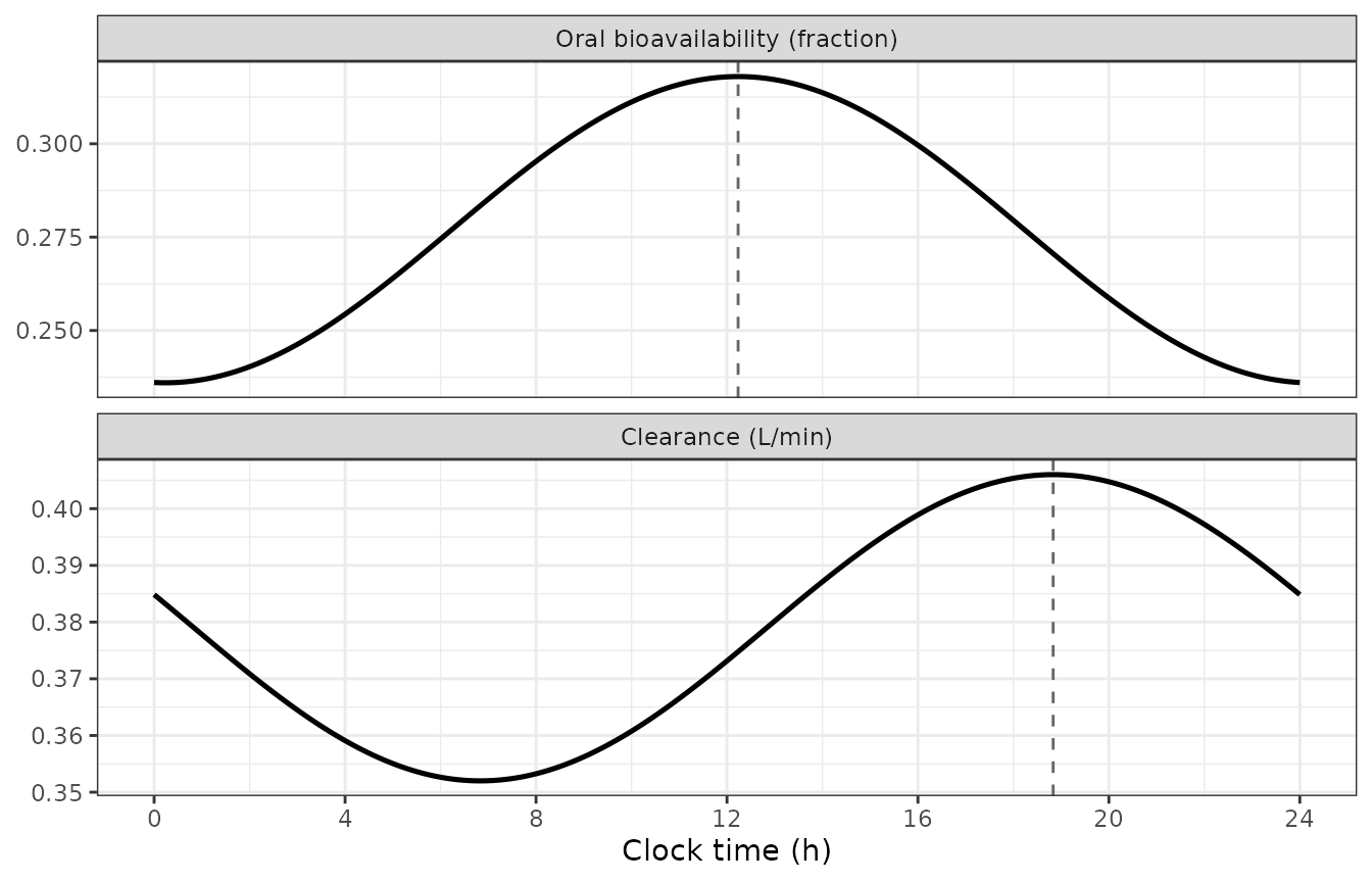
Replicates Figure 4 of van Rongen 2015: 24-hour fluctuation in oral bioavailability (upper) and clearance (lower) under the final model. Dashed vertical lines mark the estimated acrophases, 12:14 for bioavailability and 18:50 for clearance.
Replicating Figure 5
Figure 5 simulates a typical subject given either a 7.5 mg oral dose or a 2 mg intravenous bolus at each of the six administration times. The paper’s reading of that figure is threefold: oral concentrations are higher after late-morning / early-afternoon dosing (10:00 and 14:00) than after late-evening / early-night dosing (22:00 and 02:00); time to maximum concentration is shorter at 14:00; and the intravenous profiles barely move across the day.
fig5_arm <- function(tclock, route) {
  amt <- if (route == "Oral 7.5 mg") 7.5 else 2
  cmt <- if (route == "Oral 7.5 mg") "depot" else "central"
  e <- rxode2::et(amt = amt, cmt = cmt, time = 0)
  e <- rxode2::et(e, sort(unique(c(seq(0, 60, 1), seq(60, 720, 5)))), cmt = "central")
  d <- as.data.frame(e)
  d$TCLOCK <- tclock; d$OCC <- 1
  d$ROUTE_IV <- as.integer(cmt == "central")
  d$route <- route
  d$admin <- sprintf("%02d:00", tclock)
  d
}
fig5_ev <- bind_rows(lapply(c("Oral 7.5 mg", "IV 2 mg bolus"),
                            function(r) bind_rows(lapply(admin_times, fig5_arm, route = r))))
fig5_ev$id <- as.integer(factor(paste(fig5_ev$route, fig5_ev$admin)))

fig5 <- rxode2::rxSolve(typical, fig5_ev, returnType = "data.frame") |>
  left_join(distinct(fig5_ev, id, route, admin), by = "id") |>
  mutate(route = factor(route, levels = c("Oral 7.5 mg", "IV 2 mg bolus")))
#> ℹ omega/sigma items treated as zero: 'etalcl', 'etalka', 'etalfdepot', 'etaiov_fdepot_1', 'etaiov_fdepot_2', 'etaiov_fdepot_3', 'etaiov_fdepot_4', 'etaiov_fdepot_5', 'etaiov_fdepot_6'
#> Warning: multi-subject simulation without without 'omega'

ggplot(filter(fig5, !is.na(Cc)), aes(time, Cc, colour = admin)) +
  geom_line(linewidth = 0.8) +
  facet_wrap(~route, scales = "free_y") +
  labs(x = "Time after dose (min)", y = "Midazolam (ug/L)", colour = "Dosed at") +
  theme_bw()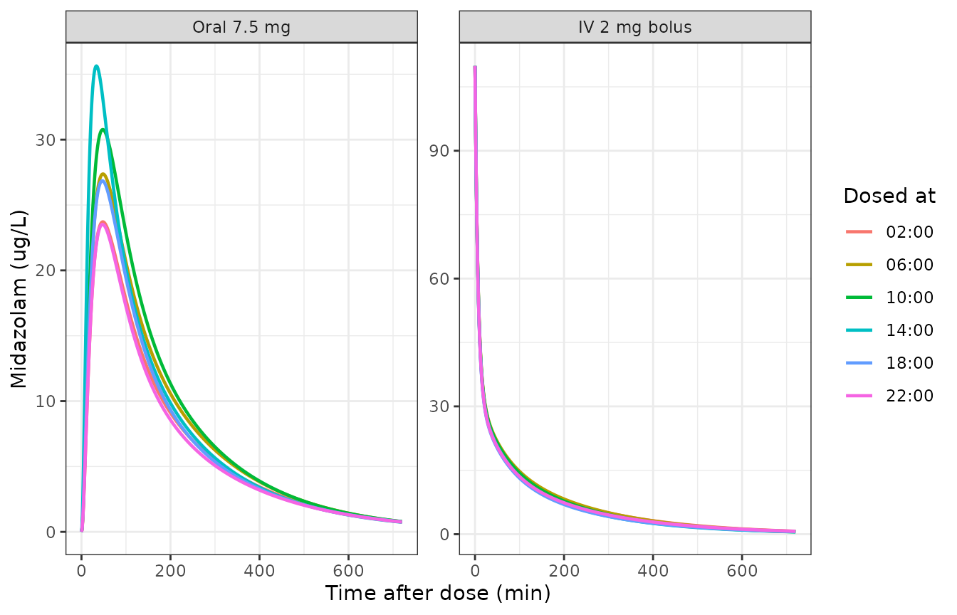
Replicates Figure 5 of van Rongen 2015: population-predicted midazolam concentrations after a 7.5 mg oral dose (left) and a 2 mg intravenous bolus (right) in a typical subject dosed at six clock times.
fig5_sum <- fig5 |>
  filter(!is.na(Cc)) |>
  group_by(route, admin) |>
  summarise(Cmax = max(Cc), Tmax = time[which.max(Cc)],
            AUC0_720 = sum(diff(time) * (head(Cc, -1) + tail(Cc, -1)) / 2),
            .groups = "drop")
knitr::kable(fig5_sum, digits = c(0, 0, 2, 0, 1),
caption = "Typical-value exposure by route and administration time, from the Figure 5 replication. These are deterministic (zeroRe) solves, so the checks below are exact rather than cohort-derived.")| route | admin | Cmax | Tmax | AUC0_720 |
|---|---|---|---|---|
| Oral 7.5 mg | 02:00 | 23.71 | 48 | 4835.8 |
| Oral 7.5 mg | 06:00 | 27.37 | 48 | 5540.9 |
| Oral 7.5 mg | 10:00 | 30.77 | 48 | 5998.4 |
| Oral 7.5 mg | 14:00 | 35.63 | 34 | 5777.1 |
| Oral 7.5 mg | 18:00 | 26.85 | 47 | 5112.6 |
| Oral 7.5 mg | 22:00 | 23.52 | 47 | 4648.0 |
| IV 2 mg bolus | 02:00 | 109.89 | 0 | 5368.8 |
| IV 2 mg bolus | 06:00 | 109.89 | 0 | 5432.1 |
| IV 2 mg bolus | 10:00 | 109.89 | 0 | 5211.9 |
| IV 2 mg bolus | 14:00 | 109.89 | 0 | 4947.3 |
| IV 2 mg bolus | 18:00 | 109.89 | 0 | 4887.8 |
| IV 2 mg bolus | 22:00 | 109.89 | 0 | 5089.1 |
oral <- filter(fig5_sum, route == "Oral 7.5 mg")
ivb  <- filter(fig5_sum, route == "IV 2 mg bolus")
getv <- function(tab, col, hh) {
  v <- tab[[col]][tab$admin == hh]
  if (length(v) != 1L) stop("no unique row for ", hh)
  v
}

stopifnot(
  # Paper: concentrations after 10:00 and 14:00 dosing exceed those after
  # 22:00 and 02:00 dosing.
  min(getv(oral, "Cmax", "10:00"), getv(oral, "Cmax", "14:00")) >
    max(getv(oral, "Cmax", "22:00"), getv(oral, "Cmax", "02:00")),
  min(getv(oral, "AUC0_720", "10:00"), getv(oral, "AUC0_720", "14:00")) >
    max(getv(oral, "AUC0_720", "22:00"), getv(oral, "AUC0_720", "02:00")),
  # Paper: Tmax is shorter when midazolam is administered at 14:00.
  getv(oral, "Tmax", "14:00") < min(oral$Tmax[oral$admin != "14:00"]),
  # Paper: the intravenous profiles show almost no variation over the day.
  # Cmax for a bolus is dose/Vc exactly and cannot vary at all; AUC varies
  # only through the clearance cosine, whose peak-to-trough span is 14.4%.
  all(abs(ivb$Cmax - 2000 / 18.2) < 1e-6),
  diff(range(ivb$AUC0_720)) / mean(ivb$AUC0_720) < 0.15,
  # ... and the oral spread is much larger than the intravenous spread.
  diff(range(oral$AUC0_720)) / mean(oral$AUC0_720) > 0.20
)
PKNCA validation against the published parameters
van Rongen 2015 report no NCA table, so the reference values here are
derived from the paper’s own printed parameters. Two exact identities
are available once the circadian terms are switched off, which is what
the ini() override below does: with a constant clearance,
AUC(0-inf) = Dose / CL for an intravenous dose and
AUC(0-inf) = F * Dose / CL for an oral dose, and for an
intravenous bolus Cmax = Dose / Vc.
Switching the amplitudes off is essential for these to be identities rather than approximations – with a time-varying clearance neither holds exactly. Both reference sides are written from the printed Table 2 numbers rather than read back out of the model, so the gate can actually go red.
flat <- rxode2::ini(rxode2::zeroRe(mod), amp_cl = 0, amp_fdepot = 0)
#> Warning: No sigma parameters in the model
#> Warning: some etas defaulted to non-mu referenced, possible parsing error: etaiov_fdepot_1, etaiov_fdepot_2, etaiov_fdepot_3, etaiov_fdepot_4, etaiov_fdepot_5, etaiov_fdepot_6
#> as a work-around try putting the mu-referenced expression on a simple line
#> ℹ change initial estimate of `amp_cl` to `0`
#> ℹ change initial estimate of `amp_fdepot` to `0`

nca_grid <- sort(unique(c(seq(0, 5, by = 0.05), seq(5, 120, by = 0.5),
                          seq(120, 720, by = 2), seq(720, 4320, by = 10))))
nca_arms <- tibble::tribble(
  ~treatment,   ~amt, ~cmt,
  "Oral 2 mg",   2,   "depot",
  "IV 1 mg",     1,   "central",
  "IV 2 mg",     2,   "central"
)
nca_events <- bind_rows(lapply(seq_len(nrow(nca_arms)), function(i) {
  e <- rxode2::et(amt = nca_arms$amt[i], cmt = nca_arms$cmt[i], time = 0)
  e <- rxode2::et(e, nca_grid, cmt = "central")
  d <- as.data.frame(e)
  d$id <- i
  d$treatment <- nca_arms$treatment[i]
  d$TCLOCK <- 14; d$OCC <- 1
  d$ROUTE_IV <- as.integer(nca_arms$cmt[i] == "central")
  d
}))

nca_sim <- rxode2::rxSolve(flat, nca_events, returnType = "data.frame") |>
  left_join(distinct(nca_events, id, treatment), by = "id")
#> ℹ omega/sigma items treated as zero: 'etalcl', 'etalka', 'etalfdepot', 'etaiov_fdepot_1', 'etaiov_fdepot_2', 'etaiov_fdepot_3', 'etaiov_fdepot_4', 'etaiov_fdepot_5', 'etaiov_fdepot_6'
#> Warning: multi-subject simulation without without 'omega'

sim_nca <- nca_sim |>
  filter(!is.na(Cc)) |>
  select(id, time, Cc, treatment)

# The solve already supplies a time-zero record for every arm (post-dose for
# the bolus arms, zero for the oral arm), but guarantee it defensively.
sim_nca <- bind_rows(
  sim_nca,
  sim_nca |> distinct(id, treatment) |> mutate(time = 0, Cc = 0)
) |>
  distinct(id, treatment, time, .keep_all = TRUE) |>
  arrange(id, treatment, time)

stopifnot(all(sim_nca$Cc >= 0))

conc_obj <- PKNCA::PKNCAconc(
  sim_nca, Cc ~ time | treatment + id, concu = "ug/L", timeu = "min"
)
dose_obj <- PKNCA::PKNCAdose(
  nca_events |> filter(evid == 1L) |> select(id, time, amt, treatment),
  amt ~ time | treatment + id, doseu = "mg"
)
nca_res <- PKNCA::pk.nca(PKNCAdata(
  conc_obj, dose_obj,
  intervals = data.frame(start = 0, end = Inf,
                         cmax = TRUE, aucinf.obs = TRUE, half.life = TRUE)
))
CL_PAPER <- 0.379   # L/min,  Table 2 CLmesor
VC_PAPER <- 18.2    # L,      Table 2 Vcentral
F_PAPER  <- 0.277   # ,       Table 2 Fmesor

published <- tibble::tribble(
  ~treatment,  ~cmax,                   ~aucinf.obs,
  "Oral 2 mg", NA_real_,                F_PAPER * 2000 / CL_PAPER,
  "IV 1 mg",   1000 / VC_PAPER,         1000 / CL_PAPER,
  "IV 2 mg",   2000 / VC_PAPER,         2000 / CL_PAPER
)

cmp <- nlmixr2lib::ncaComparisonTable(
  simulated     = nca_res,
  reference     = published,
  by            = "treatment",
  params        = c("cmax", "aucinf.obs"),
  units         = c(cmax = "ug/L", aucinf.obs = "ug*min/L"),
  tolerance_pct = 20
)
knitr::kable(
  cmp,
  caption = "Simulated NCA versus the closed-form values implied by the published CL, Vc and F, with the circadian amplitudes switched off. Oral Cmax has no closed form and is left blank on the reference side. * marks rows differing by more than 20%."
)| NCA parameter | treatment | Reference | Simulated | % diff |
|---|---|---|---|---|
| Cmax (ug/L) | Oral 2 mg | — | 8.44 | — |
| Cmax (ug/L) | IV 1 mg | 54.9 | 54.9 | -0.0% |
| Cmax (ug/L) | IV 2 mg | 110 | 110 | -0.0% |
| AUC0-∞ (obs) (ug*min/L) | Oral 2 mg | 1460 | 1460 | -0.0% |
| AUC0-∞ (obs) (ug*min/L) | IV 1 mg | 2640 | 2640 | +0.0% |
| AUC0-∞ (obs) (ug*min/L) | IV 2 mg | 5280 | 5280 | +0.0% |
getnca <- function(trt, param) {
  v <- nca_res$result$PPORRES[nca_res$result$treatment == trt &
                                nca_res$result$PPTESTCD == param]
  if (length(v) != 1L) stop("no unique NCA result for ", trt, " / ", param)
  v
}

auc_po  <- getnca("Oral 2 mg", "aucinf.obs")
auc_iv1 <- getnca("IV 1 mg",   "aucinf.obs")
auc_iv2 <- getnca("IV 2 mg",   "aucinf.obs")

# Deterministic solves of a linear model against exact identities, so these
# tolerances reflect trapezoidal and lambda.z error only -- nothing here is
# cohort-derived and nothing varies with solver thread count.
stopifnot(
  abs(auc_iv1 / (1000 / CL_PAPER)            - 1) < 0.005,
  abs(auc_iv2 / (2000 / CL_PAPER)            - 1) < 0.005,
  abs(auc_po  / (F_PAPER * 2000 / CL_PAPER)  - 1) < 0.005,
  abs(getnca("IV 1 mg", "cmax") / (1000 / VC_PAPER) - 1) < 1e-3,
  abs(getnca("IV 2 mg", "cmax") / (2000 / VC_PAPER) - 1) < 1e-3,
  # Dose proportionality of the linear disposition.
  abs(auc_iv2 / auc_iv1 - 2) < 0.005
)

# Recovering absolute bioavailability the way the semi-simultaneous design is
# meant to be read: the dose-normalised oral-to-intravenous AUC ratio.
f_recovered <- (auc_po / 2) / (auc_iv2 / 2)
stopifnot(abs(f_recovered - F_PAPER) < 0.005)
sprintf("Bioavailability recovered by cross-route NCA: %.4f (Table 2 Fmesor %.3f).",
        f_recovered, F_PAPER)
#> [1] "Bioavailability recovered by cross-route NCA: 0.2770 (Table 2 Fmesor 0.277)."
Virtual cohort and the study design
The last check simulates the study as it was actually run – a 2 mg oral dose followed 150 minutes later by a 1 mg intravenous bolus – at each of the six administration times, with the full random-effect structure (IIV on CL, Ka and F, plus inter-occasion variability on F). The six arms are re-seeded identically so each arm draws the same subjects, making the across-arm contrast paired rather than a race between six independent cohorts.
N_PER_ARM <- 100L
SAMPLES <- c(0, 15, 30, 45, 58, 65, 70, 75, 80, 90, 120, 148,
             155, 165, 180, 210, 240, 270, 330, 390)

sim_arm <- function(tclock, occ) {
  ev <- rxode2::et(amt = 2, cmt = "depot", time = 0)
  ev <- rxode2::et(ev, amt = 1, cmt = "central", time = 150)
  ev <- rxode2::et(ev, SAMPLES, cmt = "central")
  ev <- rxode2::et(ev, id = seq_len(N_PER_ARM))
  d <- as.data.frame(ev)
  d$TCLOCK <- tclock
  d$OCC <- occ
  d$ROUTE_IV <- as.integer(d$time >= 150)
  # Common random numbers: each arm redraws the same cohort, so the
  # across-arm contrast is within-subject rather than between-cohort.
  rxode2::rxSetSeed(20150724)
  out <- rxode2::rxSolve(mod, d, returnType = "data.frame")
  out$admin <- sprintf("%02d:00", tclock)
  out
}
cohort <- bind_rows(Map(sim_arm, admin_times, seq_along(admin_times)))
cohort_q <- cohort |>
  filter(!is.na(Cc)) |>
  group_by(admin, time) |>
  summarise(med = median(Cc), lo = quantile(Cc, 0.025), hi = quantile(Cc, 0.975),
            .groups = "drop")

ggplot(cohort_q, aes(time, med)) +
  geom_ribbon(aes(ymin = lo, ymax = hi), alpha = 0.25, fill = "steelblue") +
  geom_line(linewidth = 0.8, colour = "steelblue4") +
  geom_vline(xintercept = 150, linetype = "dotted", colour = "grey30") +
  facet_wrap(~admin) +
  labs(x = "Time after oral dose (min)", y = "Midazolam (ug/L)") +
  theme_bw()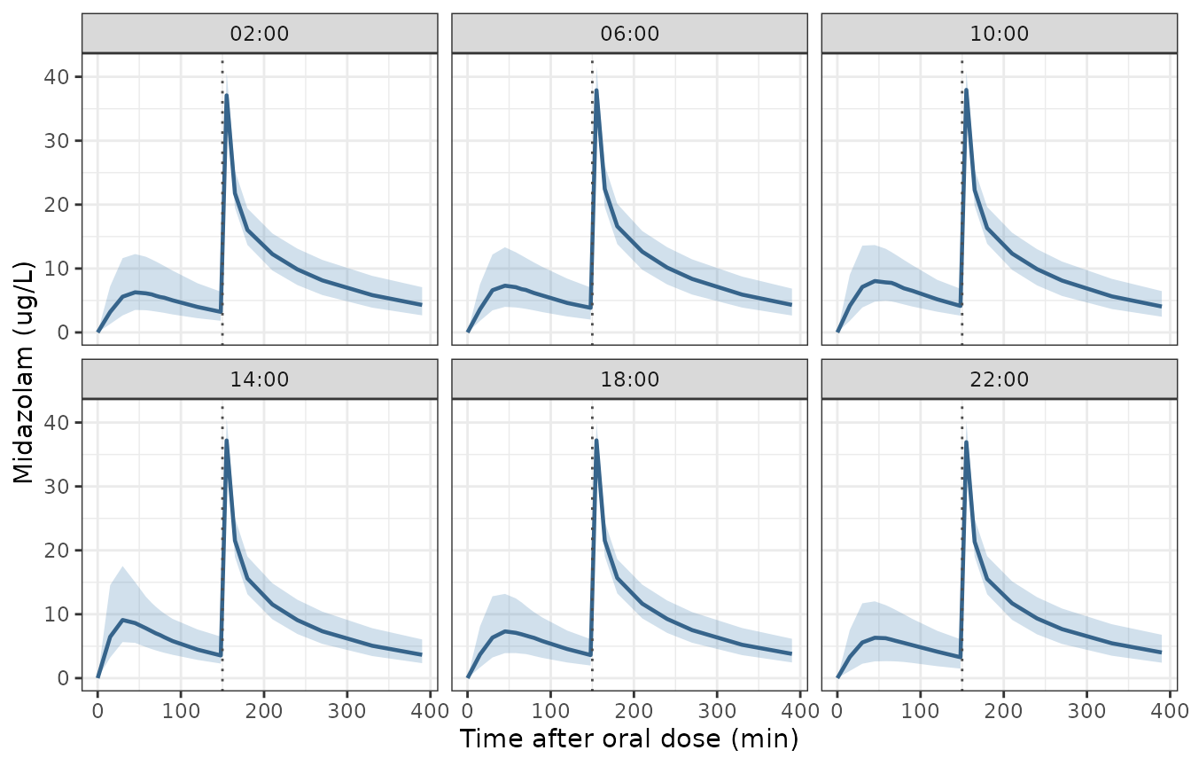
Simulated midazolam concentration-time profiles for the semi-simultaneous study design (2 mg oral at t = 0, 1 mg intravenous at t = 150 min) at each of the six administration times, in the style of the Figure 3 visual predictive checks. Lines are the cohort median and ribbons the 2.5th-97.5th percentile interval of the individual predictions Cc, so they carry the inter-individual and inter-occasion variability but not the residual error.
# Pre-intravenous window only, so the contrast is driven by the oral dose.
oral_phase <- cohort |>
  filter(!is.na(Cc), time < 150) |>
  group_by(admin, id) |>
  summarise(Cmax = max(Cc), .groups = "drop") |>
  group_by(admin) |>
  summarise(medCmax = median(Cmax), .groups = "drop")
knitr::kable(oral_phase, digits = 2,
caption = "Cohort median oral-phase Cmax (samples before the intravenous dose) by administration time, 100 subjects per arm with common random numbers.")| admin | medCmax |
|---|---|
| 02:00 | 6.36 |
| 06:00 | 7.39 |
| 10:00 | 8.04 |
| 14:00 | 9.10 |
| 18:00 | 7.41 |
| 22:00 | 6.43 |
day_med   <- mean(oral_phase$medCmax[oral_phase$admin %in% c("10:00", "14:00")])
night_med <- mean(oral_phase$medCmax[oral_phase$admin %in% c("22:00", "02:00")])

stopifnot(
  # Cohort-derived, so this is a magnitude claim with headroom, not a bare
  # ordering. Realised 1.340 / 1.414 / 1.399 / 1.329 at 1 / 2 / 4 / 16 solver
  # threads, so 1.15 sits well below the range rxSetSeed can produce (the seed
  # fixes the draw per thread count, not across thread counts). It still
  # breaks on a mis-transcribed amplitude, mesor or acrophase, all of which
  # collapse the ratio towards 1.
  day_med / night_med > 1.15,
  nrow(oral_phase) == 6L,
  all(is.finite(oral_phase$medCmax))
)
sprintf("Day (10:00, 14:00) versus night (22:00, 02:00) median oral Cmax ratio: %.2f.",
        day_med / night_med)
#> [1] "Day (10:00, 14:00) versus night (22:00, 02:00) median oral Cmax ratio: 1.34."
Assumptions and deviations
File name. This paper collides with
vanRongen_2015_midazolam.R, an unrelated van Rongen 2015 midazolam model (doi:10.1111/bcp.12693, parent and metabolites in overweight and obese adolescents). The two are different papers in different journals with different populations, so this extraction takes the descriptive suffix_circadianrather than renaming the already published file – matching the sibling-pair convention already used for midazolam in this library (Cella_2012_midazolam_children_adolescents/Cella_2012_midazolam_infants_adults,Kim_2026_midazolam_ecmo/Kim_2026_midazolam_postecmo,Hyland_2009_midazolam_hlm/Hyland_2009_midazolam_rugt1a4).The 14:00 factor applies to both absorption steps. Table 2 reports
Ka = Ktras a single estimated row and a separate row “Fraction Ka at 14:00”. Because the transit and absorption rate constants are one estimated quantity, the 1.41 factor is applied to that shared constant, so both steps of the absorption chain speed up together and Tmax scales by 1/1.41. The paper does not print the$PKcode, so a reading in which only the transit-to-central step is accelerated cannot be formally excluded; the shared-constant reading is the one consistent with the paper’s ownKa = Ktrnotation and with its statement that “the time to maximum concentration (Tmax) is shorter when midazolam is administered at 14:00”.TCLOCKis supplied time-fixed. The paper’s cosines are driven by minutes after midnight. The model reconstructs that asclockTime = TCLOCK * 60 + time, withTCLOCKthe wall-clock hour at model time zero. Supplying a wall-clock column per record instead would be wrong here: a 0-24 column wraps at midnight and rxode2’s linear covariate interpolation would sweep backwards through an entire day across the wrap.Residual-error record assignment. Table 2 reports separate proportional residual errors for the oral (18.0%) and intravenous (15.4%) data, but the paper does not state how individual records were assigned to the two strata. In a semi-simultaneous design the post-intravenous samples carry superimposed oral and intravenous contributions, so the assignment cannot be read off the source. This vignette and the model take the only record-level split the design admits:
ROUTE_IV = 0on the samples drawn between the oral dose and the intravenous dose (0-148 min) andROUTE_IV = 1on those drawn afterwards (155 min onward). Any user simulating a single route should setROUTE_IVconstant at 0 (oral) or 1 (intravenous).Six inter-occasion slots. Table 2 reports one inter-occasion variability magnitude for bioavailability. rxode2 cannot simulate the
eta ~ var | OCCform, so it is expanded into six occasion-multiplexed slots – one per administration occasion, which is how the paper defines the occasion – with occasions 2-6 held at occasion 1’s variance, the equivalent of NONMEM$OMEGA BLOCK(1) SAME.IIV scale. Table 2 reports interindividual and interoccasion variability as CV percentages for random effects the Methods describe as log-normally distributed, so the variances are encoded as
omega^2 = log(1 + CV^2). At these magnitudes the alternative readingomega = CVdiffers in the fourth decimal place and changes no conclusion in this vignette.The 1.46 factor in the Results text is not the final estimate. The Results paragraph on the absorption rate constant quotes a multiplication factor of 1.46 “resulting in an absorption rate constant of 0.08 min-1”. That value comes from the intermediate model that still carried inter-occasion variability on Ka, which was then removed for 55% eta-shrinkage. The final model’s factor is the 1.41 of Table 2, which is also the value quoted in the Abstract and the Discussion, and it is the one used here.
The rejected half-sine alternative is not implemented. Paper Equations 3 and 4 describe a half-cycle sine parameterisation of the 14:00 absorption peak (peak 14:59, amplitude 0.056 1/min, onset 14:12, offset 15:45). The authors rejected it as very sensitive to initial estimates and not a significant improvement over the multiplication factor, so only the selected multiplication-factor form is packaged.
No covariates beyond the clock. The study enrolled a deliberately narrow population (healthy Caucasian men, 18-27 years, BMI 18.8-25.8), and no demographic covariate was retained in the final model. Extrapolation outside that population is not supported by this paper.
Errata
No erratum, corrigendum, or author correction was located for this article. Supplementary Table 1 and Supplementary Figures 1-3, referenced by the paper, contain the sequential model-building objective function values, the shrinkage diagnostics, and goodness-of-fit plots; none of them carries a final-model parameter value, so every number in the packaged model comes from Table 2 of the main text.