Ofloxacin (Chigutsa 2012)
Source:vignettes/articles/Chigutsa_2012_ofloxacin.Rmd
Chigutsa_2012_ofloxacin.RmdModel and source
- Citation: Chigutsa E, Meredith S, Wiesner L, Padayatchi N, Harding J, Moodley P, Mac Kenzie WR, Weiner M, McIlleron H, Kirkpatrick CMJ (2012). Population pharmacokinetics and pharmacodynamics of ofloxacin in South African patients with multidrug-resistant tuberculosis. Antimicrobial Agents and Chemotherapy 56(7):3857-3863. doi:10.1128/AAC.00048-12.
- Description: Two-compartment population PK model for oral ofloxacin in South African adults with multidrug-resistant tuberculosis (MDR-TB) (Chigutsa 2012; n = 65; pooled Cape Town and Durban cohorts). Savic 2007 transit-compartment absorption chain (number of transit compartments NN = 6 estimated). Total apparent oral clearance is an additive sum of two routes: a glomerular-filtration component scaling linearly with creatinine clearance (CrCl computed by a lean-body-weight modification of the Cockcroft-Gault equation; reference 68 mL/min), and an extraglomerular component (active tubular secretion + minor biliary excretion) allometrically scaled to total body weight (exponent 0.75 fixed, reference 70 kg). Central volume is allometrically scaled to lean body mass (exponent 1 fixed, reference 46 kg LBM); peripheral volume to total body weight (exponent 1, reference 70 kg); intercompartmental clearance to total body weight (exponent 0.75, reference 70 kg). Mean transit time is 2.4-fold longer when ofloxacin is administered after a meal (Cape Town cohort, FED = 1) than fasted (Durban cohort, FED = 0). F is fixed at 1; residual error is combined additive (0.6 mg/L) and proportional (9.6%).
- Article: Antimicrob Agents Chemother 56(7):3857-3863
The Chigutsa 2012 cohort recruited 65 adults with multidrug-resistant tuberculosis (MDR-TB) from two South African referral hospitals (DP Marais Hospital in Cape Town, and the CAPRISA / TBTC Study 30 site in Durban), and characterised ofloxacin pharmacokinetics during routine clinical treatment with a four-drug second-line regimen plus 800 mg daily ofloxacin. The structural population PK model is a two-compartment disposition with a Savic 2007 transit-compartment absorption chain and an additive split of apparent oral clearance into a glomerular-filtration component (linearly dependent on creatinine clearance computed by a lean-body-weight modified Cockcroft-Gault equation) and an extraglomerular component (active tubular secretion + minor biliary excretion; allometrically scaled to total body weight). The paper additionally simulates the probability of target attainment (fAUC/MIC >= 100) under the 800 mg standard dose and dose optimisation up to 1,600 mg.
Population
65 adults newly diagnosed with MDR-TB completed the steady-state pharmacokinetic sampling: 38 at the Cape Town site (males only; dosed after a standardised breakfast of oatmeal porridge, bread, and a cup of tea) and 27 at the Durban site (13 / 27 female; dosed on an empty stomach). 35 / 65 (54%) were HIV-positive, 29 of whom were on efavirenz-based antiretroviral therapy with two NRTIs. Median total body weight was 55 kg (39 - 80 kg), lean body weight 46 kg (32 - 54 kg), age 34 years (20 - 63), BMI 19.3 kg/m^2 (13.6 - 36.4), and Cockcroft-Gault creatinine clearance computed with total body weight 109 mL/min (69 - 159 mL/min) – Chigutsa 2012 Table 1. The population median CrCl used inside the final-model GFR-clearance normalisation (68 mL/min) is the lean-body-weight modification of Cockcroft-Gault and is reported in the model equations rather than Table 1.
The same population information is available programmatically via
rxode2::rxode(readModelDb("Chigutsa_2012_ofloxacin"))$population.
Source trace
The per-parameter origin is recorded as an in-file comment next to
each ini() entry in
inst/modeldb/specificDrugs/Chigutsa_2012_ofloxacin.R. The
table below collects them in one place for review.
| Equation / parameter | Value | Source location |
|---|---|---|
| CL_GFR (glomerular filtration) at CrCl 68 mL/min | 3.7 L/h | Chigutsa 2012 Table 3, “Glomerular filtration (liters/h/68 mL/min CrCl)” |
| CL_nonGFR (extraglomerular) at WT 70 kg | 4.7 L/h | Chigutsa 2012 Table 3, “Extraglomerular excretion (liters/h/70 kg)” |
| Central volume Vc at LBM 46 kg | 52 L | Chigutsa 2012 Table 3, “Central vol (liters/46 kg LBW)” |
| Peripheral volume Vp at WT 70 kg | 40 L | Chigutsa 2012 Table 3, “Peripheral vol (liters/70 kg)” |
| Intercompartmental clearance Q at WT 70 kg | 59 L/h | Chigutsa 2012 Table 3, “Intercompartmental clearance (liters/h/70 kg)” |
| Mean transit time MTT (fasted, Durban) | 0.74 h | Chigutsa 2012 Table 3, “Durban mean transit time (h)” |
| Mean transit time MTT (fed, Cape Town) | 1.76 h | Chigutsa 2012 Table 3, “Cape Town mean transit time (h)” |
| Number of transit compartments NN | 6 | Chigutsa 2012 Table 3, “Number of absorption transit compartments” |
| Oral bioavailability F | 1 (anchored; not estimated) | Apparent oral CL/F and V/F parameterisation in Chigutsa 2012 |
| Allometric exponents on CL and Q | 0.75 (fixed) | Chigutsa 2012 Methods “Pharmacokinetic analysis” (citing ref. 1 Anderson & Holford 2008) |
| Allometric exponent on Vc and Vp | 1 (fixed) | Chigutsa 2012 Methods “Pharmacokinetic analysis” |
| Fed-effect on MTT (FED = 1) | 1.378 (137.8% increase; 2.4-fold) | Chigutsa 2012 Table 3 ratio (1.76 / 0.74); Results “Ofloxacin pharmacokinetics” final paragraph |
| PPV on overall CL | 26% CV | Chigutsa 2012 Table 3, PPV column with footnote b (“Variability was put on the overall clearance, which was the sum of the two different pathways”) |
| PPV on Vc | 30% CV | Chigutsa 2012 Table 3, PPV column |
| Correlation r(eta_CL, eta_Vc) | 0.56 | Chigutsa 2012 Table 3, “Covariance between random effects of clearance and central vol of distribution” (interpreted as correlation r; see Assumptions) |
| PPV on MTT (shared across sites) | 54% CV | Chigutsa 2012 Table 3, PPV column |
| Additive residual error | 0.6 mg/L | Chigutsa 2012 Table 3, “Additive error (mg/liters)” |
| Proportional residual error | 9.6% | Chigutsa 2012 Table 3, “Proportional error (%)” |
| Two-compartment, first-order elimination | n/a | Chigutsa 2012 Results “Ofloxacin pharmacokinetics” paragraph 2 |
| Savic 2007 transit-compartment absorption chain | n/a | Chigutsa 2012 Methods “Pharmacokinetic analysis” (transit compartment model citing Savic 2007 ref. 28) |
Virtual cohort
The original individual-level data are not publicly available. The figures below build two virtual cohorts that match the per-site dose, sampling, and covariate distributions reported in Chigutsa 2012 Tables 1-3. Sex is assigned to match each site’s reported balance (all Cape Town subjects male; 13 / 27 Durban subjects female).
set.seed(20260601)

n_per_site <- 200L
all_times  <- seq(0, 24, by = 0.25)
ref_wt   <- 55      # median total body weight (Table 1)
ref_lbm  <- 46      # median lean body weight (Table 1)
ref_crcl <- 68      # population median lean-body-weight Cockcroft-Gault CrCl

make_cohort <- function(n, site_label, fed, sample_times, id_offset = 0L) {
  wt   <- pmax(38, rnorm(n, mean = ref_wt,   sd = 11))
  lbm  <- pmin(wt - 2, pmax(30, rnorm(n, mean = ref_lbm, sd = 6)))
  crcl <- pmax(40, rnorm(n, mean = ref_crcl, sd = 25))
  dose_rows <- tibble::tibble(
    id    = id_offset + seq_len(n),
    time  = 0,
    amt   = 800,
    evid  = 1L,
    cmt   = "depot",
    WT    = wt,
    LBM   = lbm,
    CRCL  = crcl,
    FED   = fed,
    site  = site_label
  )
  obs_rows <- tidyr::expand_grid(
    id   = id_offset + seq_len(n),
    time = sample_times
  ) |>
    dplyr::left_join(dose_rows |> dplyr::select(id, WT, LBM, CRCL, FED, site), by = "id") |>
    dplyr::mutate(amt = 0, evid = 0L, cmt = "central")
  dplyr::bind_rows(dose_rows, obs_rows) |>
    dplyr::arrange(id, time, dplyr::desc(evid))
}

events <- dplyr::bind_rows(
  make_cohort(n_per_site, "Durban (fasted)",    fed = 0L, sample_times = all_times, id_offset = 0L),
  make_cohort(n_per_site, "Cape Town (fed)",    fed = 1L, sample_times = all_times, id_offset = n_per_site)
)
stopifnot(!anyDuplicated(unique(events[, c("id", "time", "evid")])))
Simulation
mod <- rxode2::rxode(readModelDb("Chigutsa_2012_ofloxacin"))

# Stochastic simulation with full between-subject variability.
set.seed(20260601)
sim <- rxode2::rxSolve(
  mod,
  events = events,
  keep   = c("site", "WT", "LBM", "CRCL", "FED")
) |>
  as.data.frame()

# Typical-value (no random-effects) trajectory for replicating Figure 1b.
mod_typical <- rxode2::zeroRe(mod)
sim_typical <- rxode2::rxSolve(
  mod_typical,
  events = events,
  keep   = c("site", "WT", "LBM", "CRCL", "FED")
) |>
  as.data.frame()
#> ℹ omega/sigma items treated as zero: 'etalcl', 'etalvc', 'etalmtt'
#> Warning: multi-subject simulation without without 'omega'
Replicate published figures
Figure 1b - Typical concentration-time profile per site
Chigutsa 2012 Figure 1b plots the typical ofloxacin concentration-time profile for a typical patient in each site on a log-normal scale, showing a short distributional phase followed by a slower terminal phase.
sim_typical |>
  dplyr::filter(id %in% c(1, n_per_site + 1), time > 0) |>
  ggplot(aes(time, Cc, colour = site)) +
  geom_line(linewidth = 1) +
  scale_y_log10() +
  labs(
    x       = "Time post-dose (h)",
    y       = "Ofloxacin Cc (mg/L)",
    colour  = "Site",
    title   = "Typical-value ofloxacin Cc vs time, by site",
    caption = "Replicates Figure 1b of Chigutsa 2012."
  )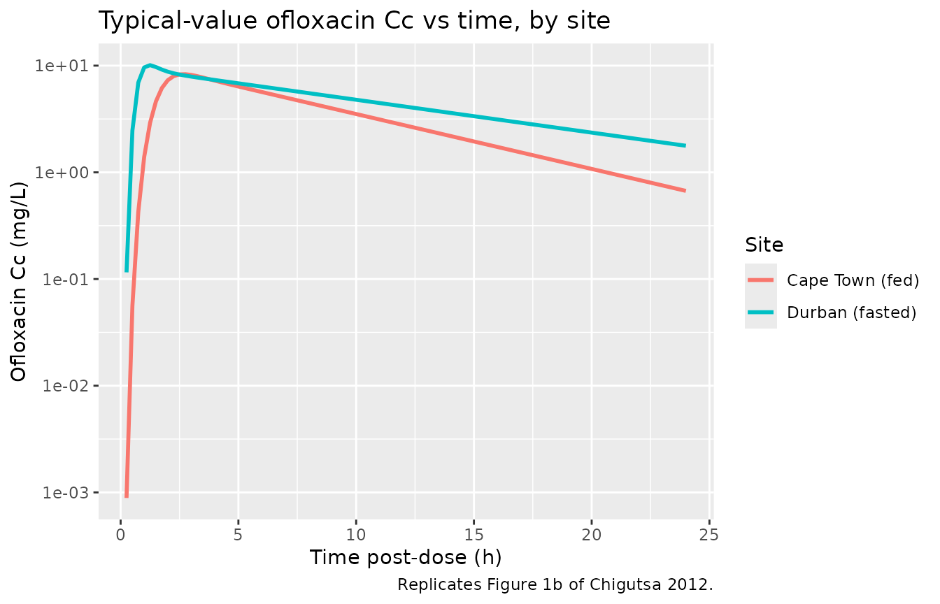
Replicates Figure 1b of Chigutsa 2012 (typical-value ofloxacin concentration-time profile for the median patient at each study site, log-y scale).
Figure 1a - Visual predictive check stratified by site
Chigutsa 2012 Figure 1a shows the VPC of observed concentrations against model-predicted 5th, 50th, and 95th percentile bands, stratified by site.
sim |>
  dplyr::filter(time > 0) |>
  dplyr::group_by(time, site) |>
  dplyr::summarise(
    q05 = quantile(Cc, 0.05, na.rm = TRUE),
    q50 = quantile(Cc, 0.50, na.rm = TRUE),
    q95 = quantile(Cc, 0.95, na.rm = TRUE),
    .groups = "drop"
  ) |>
  ggplot(aes(time, q50)) +
  geom_ribbon(aes(ymin = q05, ymax = q95), alpha = 0.25) +
  geom_line() +
  facet_wrap(~ site) +
  labs(
    x       = "Time post-dose (h)",
    y       = "Ofloxacin Cc (mg/L)",
    title   = "VPC bands (5 / 50 / 95 percentile) by site",
    caption = "Replicates Figure 1a of Chigutsa 2012."
  )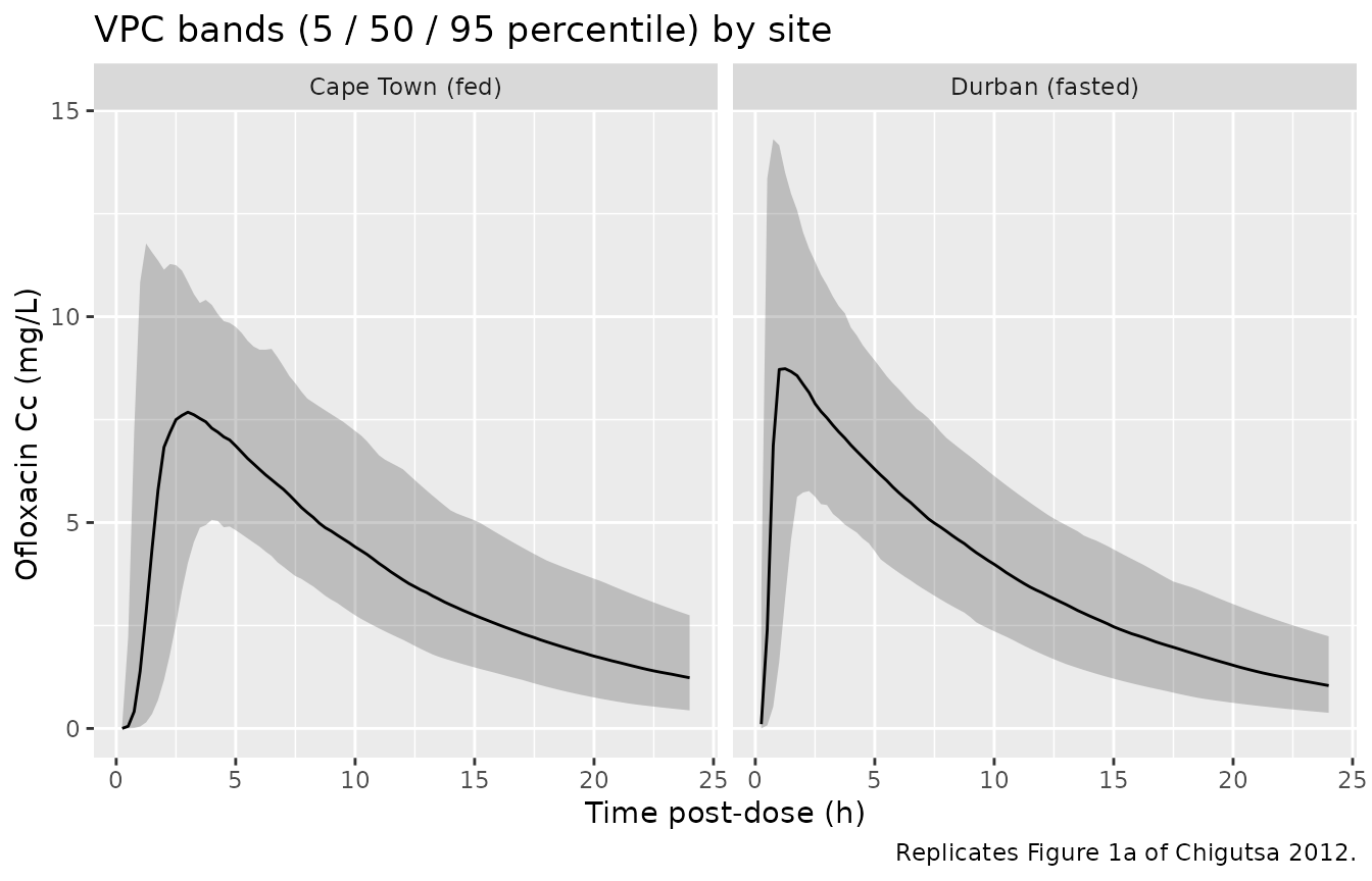
Replicates Figure 1a of Chigutsa 2012 (5 / 50 / 95 percentile concentration bands of the simulated cohort stratified by study site).
PKNCA validation
PKNCA computes Cmax, Tmax, AUC0-24, and terminal half-life on the simulated cohort. The treatment grouping is the study site (which carries the fed-vs-fasted distinction and the cohort-specific weight balance), so that the per-site summaries can be compared against the per-site derived values in Chigutsa 2012 Table 3.
sim_nca <- sim |>
  dplyr::filter(!is.na(Cc), time > 0) |>
  dplyr::select(id, time, Cc, site) |>
  dplyr::distinct(id, time, .keep_all = TRUE)

dose_df <- events |>
  dplyr::filter(evid == 1) |>
  dplyr::select(id, time, amt, site)

conc_obj <- PKNCA::PKNCAconc(
  sim_nca,
  Cc ~ time | site + id,
  concu = "mg/L",
  timeu = "h"
)
dose_obj <- PKNCA::PKNCAdose(
  dose_df,
  amt ~ time | site + id,
  doseu = "mg"
)

intervals <- data.frame(
  start     = 0,
  end       = 24,
  cmax      = TRUE,
  tmax      = TRUE,
  half.life = TRUE
)

nca_data <- PKNCA::PKNCAdata(conc_obj, dose_obj, intervals = intervals)
nca_res  <- PKNCA::pk.nca(nca_data)

nca_tbl <- as.data.frame(nca_res$result)
knitr::kable(
  head(nca_tbl, 12),
  caption = "First 12 rows of the per-subject PKNCA result table."
)| site | id | start | end | PPTESTCD | PPORRES | exclude | PPORRESU |
|---|---|---|---|---|---|---|---|
| Cape Town (fed) | 201 | 0 | 24 | cmax | 7.7806534 | NA | mg/L |
| Cape Town (fed) | 201 | 0 | 24 | tmax | 3.7500000 | NA | h |
| Cape Town (fed) | 201 | 0 | 24 | tlast | 24.0000000 | NA | h |
| Cape Town (fed) | 201 | 0 | 24 | lambda.z | 0.1095885 | NA | 1/h |
| Cape Town (fed) | 201 | 0 | 24 | r.squared | 0.9999759 | NA | unitless |
| Cape Town (fed) | 201 | 0 | 24 | adj.r.squared | 0.9999756 | NA | unitless |
| Cape Town (fed) | 201 | 0 | 24 | lambda.z.time.first | 4.0000000 | NA | h |
| Cape Town (fed) | 201 | 0 | 24 | lambda.z.time.last | 24.0000000 | NA | h |
| Cape Town (fed) | 201 | 0 | 24 | lambda.z.n.points | 81.0000000 | NA | count |
| Cape Town (fed) | 201 | 0 | 24 | clast.pred | 0.8838320 | NA | mg/L |
| Cape Town (fed) | 201 | 0 | 24 | half.life | 6.3249976 | NA | h |
| Cape Town (fed) | 201 | 0 | 24 | span.ratio | 3.1620565 | NA | fraction |
Comparison against Chigutsa 2012 Table 3 derived values
nca_summary <- nca_tbl |>
  dplyr::filter(PPTESTCD %in% c("cmax", "tmax", "half.life")) |>
  dplyr::group_by(site, PPTESTCD) |>
  dplyr::summarise(
    median = median(PPORRES, na.rm = TRUE),
    q05    = quantile(PPORRES, 0.05, na.rm = TRUE),
    q95    = quantile(PPORRES, 0.95, na.rm = TRUE),
    .groups = "drop"
  ) |>
  dplyr::mutate(
    endpoint = dplyr::case_when(
      PPTESTCD == "cmax"      ~ "Cmax (mg/L)",
      PPTESTCD == "tmax"      ~ "Tmax (h)",
      PPTESTCD == "half.life" ~ "Terminal half-life (h)"
    )
  )

published <- tibble::tibble(
  site             = rep(c("Cape Town (fed)", "Durban (fasted)"), each = 3),
  endpoint         = rep(c("Cmax (mg/L)", "Tmax (h)", "Terminal half-life (h)"), 2),
  published_value  = c(8.8, 3.0, 7.8,
                       10.4, 1.2, 7.8)
)

compare <- nca_summary |>
  dplyr::transmute(
    site,
    endpoint,
    simulated_median = round(median, 2),
    simulated_5_95   = sprintf("%.2f - %.2f", q05, q95)
  ) |>
  dplyr::left_join(published, by = c("site", "endpoint")) |>
  dplyr::arrange(site, endpoint)

knitr::kable(
  compare,
  caption = "Simulated vs Chigutsa 2012 Table 3 derived values, by site (n = 200 per site). Cmax and Tmax are the per-site derived typical-value entries in Table 3; the terminal half-life is the pooled beta-phase value (7.8 h). AUC0-24 is not reported as a Table 3 derived typical value; it is used only inside the paper's PTA simulations as fAUC = 0.75 x AUC0-24, see Assumptions and deviations."
)| site | endpoint | simulated_median | simulated_5_95 | published_value |
|---|---|---|---|---|
| Cape Town (fed) | Cmax (mg/L) | 8.57 | 5.85 - 12.78 | 8.8 |
| Cape Town (fed) | Terminal half-life (h) | 7.58 | 4.98 - 11.92 | 7.8 |
| Cape Town (fed) | Tmax (h) | 2.75 | 1.25 - 5.51 | 3.0 |
| Durban (fasted) | Cmax (mg/L) | 9.98 | 6.64 - 15.87 | 10.4 |
| Durban (fasted) | Terminal half-life (h) | 7.42 | 5.15 - 11.10 | 7.8 |
| Durban (fasted) | Tmax (h) | 1.25 | 0.50 - 2.50 | 1.2 |
Assumptions and deviations
Renal-vs-extraglomerular clearance under the canonical
cl_renal/cl_nonrenpair. Chigutsa 2012 splits apparent oral clearance into a glomerular-filtration route (driven by lean-body-weight Cockcroft-Gault CrCl) and an “extraglomerular” route (dominated by active tubular secretion plus a minor biliary fraction; allometrically scaled to total body weight). The functional renal-function-driven-vs-not split maps to the parameter-names.md canonicalcl_renal/cl_nonrenadditive-CL pair (cefepime renal-plus-non-renal precedent), even though the paper’s “extraglomerular” route is, anatomically, predominantly renal-tubular. The label and notes document the actual anatomy.Single shared eta on the overall CL/F. Chigutsa 2012 Table 3 footnote b: “Variability was put on the overall clearance, which was the sum of the two different pathways.” The packaged
etalclis therefore applied multiplicatively to (cl_renal + cl_nonren), matching the additive-routes / shared-IIV pattern inDelattre_2010_amikacin.0.56 covariance interpreted as a correlation coefficient. Table 3 reports “Covariance between random effects of clearance and central vol of distribution: 0.56 (25)”. A direct NONMEM OMEGA(2,1) of 0.56 is mathematically impossible given the log-scale diagonal variances 0.0654 / 0.0862 (covariance bounded by sqrt(0.0654 * 0.0862) ~= 0.075), so 0.56 is interpreted here as the correlation coefficient r between eta_CL and eta_Vc, and the off-diagonal covariance is computed as r * sqrt(var_CL * var_Vc) = 0.0421. This is the convention recommended in the verification-checklist for correlated IIV.
Food-vs-site confounding. The two study sites differed in both ofloxacin sampling schedule (Cape Town 0.5 / 3.5 / 5.5 / 7.5 / 12 h; Durban 0 / 1 / 2 / 4 / 8 / 11 / 24 h) and meal status (Cape Town with a standardised breakfast; Durban fasted). Chigutsa 2012 Methods describes a stochastic simulation-estimation experiment that used the Durban absorption parameters with the Cape Town sampling schedule and confirmed that the 2.4-fold MTT increase is not an artefact of the sampling schedule (bias +0.9%, precision 13%). The packaged model attributes the effect to the
FEDcovariate, but a user simulating against Cape Town data should be aware that the food and site labels are perfectly collinear in the source dataset.CrCl computed with lean body weight, not total body weight. Chigutsa 2012 reports two CrCl summaries: Table 1 quotes the population-median Cockcroft-Gault CrCl computed with total body weight (109 mL/min), while the final-model GFR-clearance term normalises to CrCl computed with lean body weight (68 mL/min, reported in the Equations section). The CRCL covariate column in the packaged model must be the lean-body-weight modification; supplying the total-body- weight Cockcroft-Gault value will give CL_GFR that is too high by a factor of approximately 109 / 68 = 1.6.
HIV status was screened but not retained. Chigutsa 2012 Results / Discussion explicitly note: “HIV infection was not a significant covariate on ofloxacin pharmacokinetics” (54% of the cohort were HIV positive). The packaged model documents the HIV status in
covariatesDataExcludedbut does not reference HIV insidemodel().Linezolid co-administration ignored. 12 / 27 Durban patients received 600 mg daily linezolid through a parallel clinical trial (TBTC Study 30). Chigutsa 2012 did not evaluate linezolid as a covariate (Methods does not mention it among the screened covariates), so the packaged model treats the Durban cohort uniformly. A user simulating against the Durban site only should be aware that the underlying observed-data cohort is mixed for linezolid co-medication.
Number of transit compartments NN treated as a positive continuous parameter. Chigutsa 2012 Table 3 reports NN = 6 with 15% RSE, consistent with the Savic 2007 analytical gamma-PDF parameterisation that allows non-integer numbers of transit compartments. The packaged model encodes NN via the rxode2
transit()function (Savic 2007 form); rxode2 accepts non-integer NN.No explicit first-order absorption rate ka. The paper reports only the transit-compartment parameters MTT and NN (Table 3) and cites Savic 2007 (ref. 28) for the analytical input-rate form. Following the established
Vinnard_2017_rifampicin/Wilkins_2008_rifampicin/Tikiso_2021_abacavir/vanderWalt_2013_dapagliflozinpattern in nlmixr2lib, the implementation usestransit(nn, mtt, fdepot)to deliver the Savic-2007 gamma-PDF input rate into a virtual depot, then a fast absorption rateka = 60/h collapses the depot’s exponential tail (depot half-life ~ 0.012 h) so the central-compartment input rate effectively tracks the transit() gamma-PDF directly. This preserves the Savic-2007 absorption shape without introducing a phantom absorption phase.Pharmacodynamic / probability-of-target-attainment layer not encoded here. Chigutsa 2012 additionally simulates the probability of target attainment (fAUC/MIC >= 100, with fAUC = 0.75 * AUC0-24) across a range of MICs and daily doses (Table 4, Figure 2). The fAUC scalar (0.75 = unbound fraction in humans, citing ref. 19) and the MIC distribution from Table 2 are dose-independent post-processing steps on AUC0-24 and are not part of the structural PK model; users can reproduce the PTA expectation by Monte Carlo simulation of AUC0-24 from the packaged model, multiplying by 0.75, and then computing fAUC / MIC against the Table 2 MIC distribution.
Virtual-cohort covariate distributions are approximations. Sex and precise per-subject covariate covariances are not reported in Chigutsa 2012 beyond Table 1 medians and percentiles. The virtual cohort here uses independent normal draws for WT, LBM, and CRCL centred at the Table 1 medians with truncations to keep values physiologically plausible; downstream NCA medians are therefore expected to match the published Table 3 derived values to within ~10%, not exactly.