Vancomycin (Polaskova 2024)
Source:vignettes/articles/Polaskova_2024_vancomycin.Rmd
Polaskova_2024_vancomycin.RmdModel and source
Citation: Polaskova L, Murinova I, Gregorova J, Slanar O, Sima M. Vancomycin population pharmacokinetics and dosing proposal for the initial treatment in obese adult patients. Front Pharmacol. 2024;15:1364681. doi:10.3389/fphar.2024.1364681
Description: One-compartment IV-infusion population PK model for vancomycin during the INITIAL phase of therapy (first 3 days) in 138 adult obese (BMI >= 30 kg/m2) patients (Polaskova 2024). Clearance is 1.32 L/h multiplied by two UNCENTERED exponential covariate terms, exp(0.61 x eGFR) and exp(0.011 x LBM), where eGFR is the creatinine-based CKD-EPI estimate in mL/s/1.73 m2 and LBM is Boer-formula lean body mass in kg; at the cohort median covariates (eGFR 1.51, LBM 68 kg) this gives 7 L/h. The central volume is 75.0 L with NO retained covariate: the authors screened body weight, LBM, BSA and BMI against Vd and found none of them a reliable predictor in this obese cohort. Residual error is additive (constant) at 2.9 mg/L.
This is a one-compartment intravenous vancomycin model fitted to therapeutic drug monitoring data from the initial phase of therapy – the first three days – in adult obese patients. That focus is the paper’s contribution: almost every published vancomycin population PK model is built from steady-state maintenance-phase samples, so the models that exist are least informative exactly when the dosing decision matters most.
Two features make this model unusual enough to be worth calling out before any code runs.
-
The central volume carries no covariate at all. The
authors screened total body weight, lean body mass, body surface area
and body mass index against
Vdand retained none of them (Results 3.2, Figure 2A). In an obese cohort spanning 73-190 kg that is a deliberate, argued negative result, not an omission – the Discussion attributes it to weight gain in obesity being mainly adipose deposition, which a hydrophilic drug does not distribute into. -
Both clearance covariate effects are exponential in the raw,
uncentered covariate. The published form is
CL = 1.32 * exp(0.61 * eGFR) * exp(0.011 * LBM), with no reference value subtracted from either covariate.CL_pop = 1.32 L/his therefore the clearance extrapolated toeGFR = 0andLBM = 0; it is a normalisation constant, not a typical clearance, and it should not be read as one. Supplying either covariate as zero, or on the wrong unit scale, does not produce a mildly wrong clearance – it produces a clearance off by a factor of several.
Population
138 adult obese inpatients (BMI >= 30 kg/m2) at the Military University Hospital in Prague contributed 147 vancomycin serum concentrations collected between January 2013 and December 2022 (Polaskova 2024 Table 1, Results 3.1). Median (IQR) age was 65 (54-72) years, body weight 104 (95-120) kg, lean body mass 68 (55-76) kg and BMI 34.3 (32.5-38.3) kg/m2; 56 of 138 patients (40.6%) were female. Renal function skewed preserved-to-augmented: eGFR by the creatinine-based CKD-EPI equation was 1.51 (1.12-1.72) mL/s/1.73 m2, i.e. 90.6 (67.2-103.2) mL/min/1.73 m2, with 52% of patients at or above 1.5 and 5% at or above 2.13 mL/s/1.73 m2. Patients receiving renal replacement therapy or extracorporeal life support were excluded, so the model carries no information about dialysis.
Sampling was sparse and trough-dominated: 1-2 concentrations per patient, of which 124 (84.4%) were troughs drawn 0-1 h before the next dose, 11 (7.5%) were peaks drawn up to 2 h after the end of infusion, and 12 (8.2%) were mid-interval. Estimation was by SAEM in Monolix 2021R2 with a 250-replicate bootstrap for stability.
The same information is available programmatically via
rxode2::rxode(readModelDb("Polaskova_2024_vancomycin"))$population.
| Field | Value |
|---|---|
| species | human |
| n_subjects | 138 |
| n_studies | 1 |
| n_observations | 147 |
| age_range | 26-86 years |
| age_median | 65 years |
| weight_range | 73-190 kg |
| weight_median | 104 kg |
| sex_female_pct | 40.6 |
| race_ethnicity | |
| disease_state | Adult obese (BMI >= 30 kg/m2) inpatients treated for suspected or proven invasive Gram-positive infection: CNS infection 33%, sepsis 18%, orthopaedic 15%, ocular 9%, skin 6%, other (pneumonia, bacteriuria, bacteraemia, endocarditis, intra-abdominal) 19% |
| dose_range | Loading dose 1-4 g (median 2.5 g) as a 0.5-7 h (median 5 h) IV infusion in 122 of 138 patients; maintenance dose 0.5-1.5 g (median 1 g) q6h, q8h, q12h or q24h as a 1-3 h (median 2 h) IV infusion, or 1-4 g/day (median 2 g/day) by continuous infusion in 9 patients |
| regions | Czechia (single centre: Military University Hospital Prague) |
| renal_function | eGFR (CKD-EPI, creatinine) median 1.51 mL/s/1.73 m2 (IQR 1.12-1.72, range 0.17-2.47), i.e. median 90.6 mL/min/1.73 m2 (IQR 67.2-103.2, range 10.2-148.2). 52% of patients had eGFR >= 1.5 mL/s/1.73 m2 and 5% >= 2.13. Patients on renal replacement therapy or extracorporeal life support were EXCLUDED. |
| notes | Retrospective open-label observational study of routine therapeutic drug monitoring data, January 2013 to December 2022 (Methods 2.1). Baseline demographics are Polaskova 2024 Table 1. Only concentrations from the INITIAL phase of therapy – the first 3 days of treatment – were included, which is the paper’s whole point: most published vancomycin popPK models describe maintenance dosing at steady state. 147 serum concentrations from 138 patients (1-2 per patient): 11 (7.5%) peaks taken up to 2 h after the end of infusion, 124 (84.4%) troughs taken 0-1 h before the next dose, and 12 (8.2%) mid-interval samples with recorded sampling times. Assay: immunoturbidimetric KIMS on a Roche Cobas 8000, LLOQ 4.0 mg/L, measuring range 4.0-80.0 mg/L. Estimation was by SAEM in Monolix 2021R2. Model stability was checked by a 250-replicate bootstrap (Table 2); the bootstrap median for Vd_pop, 79.3 L, sits about 6% above the 75.0 L final estimate, and every other bootstrap median is within a few percent of its point estimate. |
Source trace
Every value below is also carried as an in-file comment beside its
ini() entry in
inst/modeldb/specificDrugs/Polaskova_2024_vancomycin.R.
| Equation / parameter | Value | Source location |
|---|---|---|
lvc (Vd) |
75.0 L | Table 2, Vd_pop; R.S.E. 8.66%, bootstrap median 79.3
(95% CI 77.8-80.9) |
lcl (CL at eGFR = 0, LBM = 0) |
1.32 L/h | Table 2, CL_pop; R.S.E. 19.3%, bootstrap median 1.27
(95% CI 1.24-1.31) |
e_crcl_cl |
0.61 per mL/s/1.73 m2 | Table 2, beta_CL_eGFR; R.S.E. 11.8%, bootstrap median
0.61 (95% CI 0.60-0.63) |
e_lbm_cl |
0.011 per kg | Table 2, beta_CL_LBM; R.S.E. 21.6%, bootstrap median
0.011 (95% CI 0.0108-0.0113) |
etalvc |
0.31 SD -> 0.0961 variance | Table 2, Omega_Vd; footnote defines Omega as “standard
deviation of the random effects” |
etalcl |
0.28 SD -> 0.0784 variance | Table 2, Omega_CL; same footnote |
addSd |
2.9 mg/L | Table 2, “Constant”; Results 3.2 “A constant error model was the most accurate” |
Vd = Vd_pop (no covariate) |
n/a | Results 3.2 equation block; Figure 2A; Discussion paragraph on weight-independent Vd |
CL = CL_pop * exp(b_eGFR * eGFR) * exp(b_LBM * LBM) |
n/a | Results 3.2 equation block, restated in the Discussion as
CL = 1.32 x e^(0.61 x eGFR) x e^(0.011 x LBM)
|
d/dt(central) = -kel * central |
n/a | Results 3.2 “A one-compartment model with linear elimination kinetics best-fitted vancomycin concentration-time data” |
CRCL / 60 unit conversion |
n/a | Table 1 / Table 2 report eGFR in mL/s/1.73 m2; the canonical
CRCL column is mL/min/1.73 m2 |
Reproducing the paper’s own worked example
The Discussion states the model’s answer for a subject at the cohort median covariates, which is the tightest deterministic check the paper offers:
in a patient with an LBM of 68 kg and an eGFR of 1.51 mL/s/1.73 m2 (median values in our study population), the CL of vancomycin would be estimated to be 7 L/h, which with a Vd of 75 L corresponds to a t1/2 of 7.4 h
cl_published <- function(eGFR_mL_s, LBM_kg) {
  1.32 * exp(0.61 * eGFR_mL_s) * exp(0.011 * LBM_kg)
}
cl_median  <- cl_published(1.51, 68)
thalf_median <- 0.693 * 75 / cl_median
c(CL_L_per_h = cl_median, t_half_h = thalf_median)
#> CL_L_per_h   t_half_h
#>   7.005753   7.418902

# Deterministic algebra, no RNG: assert tightly. Both the /60 unit conversion
# and any swap of the two covariate coefficients move these by many-fold.
stopifnot(
  abs(cl_median - 7.0) < 0.05,
  abs(thalf_median - 7.4) < 0.05
)
Virtual cohort
Individual data are not public. The cohort below reproduces the Table 1 marginal distributions of the two retained covariates. Lean body mass and eGFR are each drawn from a log-normal matched to the published median and interquartile range and truncated to the published range; the joint distribution (and any correlation between LBM and eGFR, which the paper does not report) is not recoverable and is assumed independent. See Assumptions and deviations.
# set.seed() seeds R's RNG only. rxode2's simulation RNG is partitioned per
# solver thread, so a CI runner with a different thread count draws a different
# cohort. Every assertion below is either RNG-free (zeroRe / closed form) or
# gated on a robust cohort summary, never on a tail value.
set.seed(20240604)

n_cohort <- 200L  # cap is 200 per arm

# Draw by inverting a piecewise-linear interpolation of the published
# five-number summary (min, Q1, median, Q3, max). A fitted log-normal was tried
# first and rejected: Table 1's eGFR quartiles are LEFT-skewed (1.51/1.12 =
# 1.35 below the median against 1.72/1.51 = 1.14 above), while a log-normal is
# right-skewed, so matching the median and IQR ratio put the simulated upper
# quartile at 1.87 against the published 1.72 and inflated the median clearance
# by 14%. Quantile interpolation reproduces the median, both quartiles and the
# range by construction; it is piecewise-uniform within each band, which is as
# much shape as five published numbers can support.
sample_from_quantiles <- function(n, q) {
  stats::approx(
    x = c(0, 0.25, 0.5, 0.75, 1), y = q,
    xout = stats::runif(n), rule = 2
  )$y
}

cohort <- tibble::tibble(
  id   = seq_len(n_cohort),
  # Table 1: LBM min 41, Q1 55, median 68, Q3 76, max 104 kg.
  LBM  = sample_from_quantiles(n_cohort, c(41, 55, 68, 76, 104)),
  # Table 1: eGFR min 0.17, Q1 1.12, median 1.51, Q3 1.72, max 2.47
  # mL/s/1.73 m2. CRCL below is the canonical mL/min/1.73 m2.
  eGFR = sample_from_quantiles(n_cohort, c(0.17, 1.12, 1.51, 1.72, 2.47))
) |>
  mutate(CRCL = eGFR * 60)

# The simulated marginals should sit close to Table 1. Medians over 200 draws
# are robust; the gate is on the median only, not on any extreme.
cohort_check <- c(
  LBM_median  = stats::median(cohort$LBM),
  eGFR_median = stats::median(cohort$eGFR)
)
cohort_check
#>  LBM_median eGFR_median
#>   66.961852    1.505347
# Realised deviations over three independent 200-subject draws: LBM -1.5% /
# +0.3% / +2.3%, eGFR -0.3% / -7.8% / +2.7%. The eGFR median wanders more
# because its lowest quantile band (0.17-1.12) is wide. 15% sits outside that
# range and still goes red on a mis-entered quantile vector, which would move
# the median by tens of percent -- do not tighten it back to the observed spread.
stopifnot(
  abs(cohort_check[["LBM_median"]] / 68 - 1) < 0.15,
  abs(cohort_check[["eGFR_median"]] / 1.51 - 1) < 0.15
)
mod <- readModelDb("Polaskova_2024_vancomycin")

# Build an IV-infusion event table as a plain data frame. Covariate columns are
# added here, not onto an rxEt object (rxode2 silently drops assignments made
# onto an rxEt). Observation rows use cmt = "central" -- the ODE state name --
# never the algebraic observable Cc, which would auto-inject a compartment slot
# and renumber the system.
make_iv_events <- function(subjects, ld_mg, ld_dur_h, md_mg, md_int_h,
                           md_dur_h, end_h, obs_grid, arm) {
  md_rows <- NULL
  if (md_mg > 0 && end_h > ld_dur_h) {
    dose_times <- seq(ld_dur_h, end_h - md_int_h, by = md_int_h)
    md_rows <- subjects |>
      tidyr::crossing(time = dose_times) |>
      mutate(amt = md_mg, rate = md_mg / md_dur_h)
  }
  doses <- bind_rows(
    if (ld_mg > 0) {
      subjects |> mutate(time = 0, amt = ld_mg, rate = ld_mg / ld_dur_h)
    },
    md_rows
  ) |>
    mutate(evid = 1L, cmt = "central")
  stopifnot(nrow(doses) > 0)

  obs <- subjects |>
    tidyr::crossing(time = obs_grid) |>
    mutate(amt = NA_real_, rate = NA_real_, evid = 0L, cmt = "central")

  bind_rows(doses, obs) |>
    mutate(arm = arm) |>
    arrange(id, time, desc(evid))
}

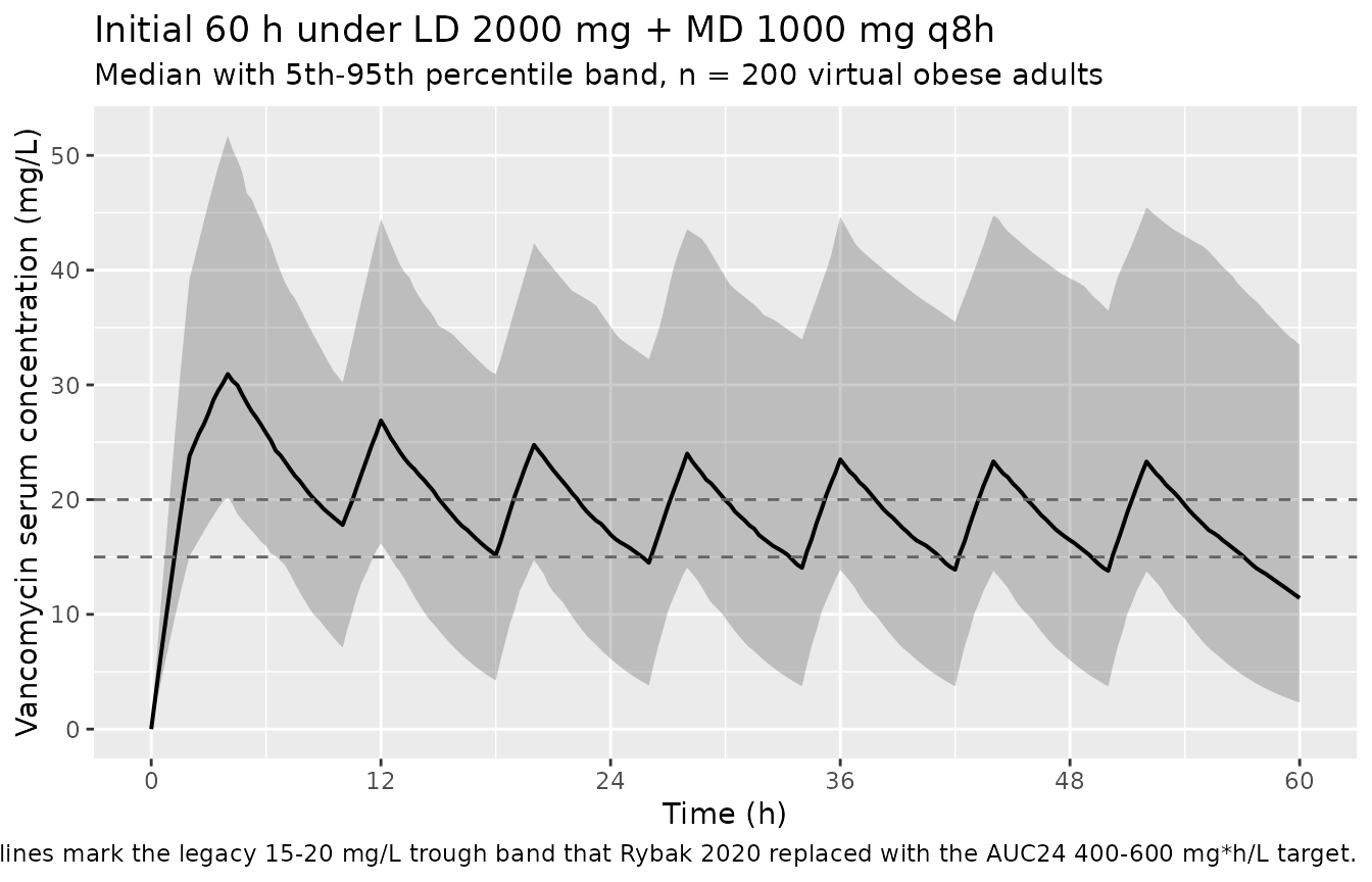
# The most frequent real-world initial regimen in this cohort: LD 2000 mg then
# MD 1000 mg q8h (Results 3.3), infused over the cohort-median 2 h. Simulated
# across the paper's own 0-60 h initial-treatment window.
obs_grid_cohort <- sort(unique(c(seq(0, 60, by = 0.25), 60)))
events_cohort <- make_iv_events(
  subjects = cohort |> select(id, CRCL, LBM),
  ld_mg = 2000, ld_dur_h = 2, md_mg = 1000, md_int_h = 8, md_dur_h = 2,
  end_h = 60, obs_grid = obs_grid_cohort,
  arm = "LD 2000 mg + MD 1000 mg q8h"
)
stopifnot(!anyDuplicated(unique(events_cohort[, c("id", "time", "evid")])))
Simulation
sim_cohort <- rxode2::rxSolve(
  mod, events = events_cohort, keep = c("arm", "CRCL", "LBM")
) |>
  as.data.frame()

# rxSolve() returns observation rows only and carries no `evid` column, so
# there is nothing to filter here.
stopifnot(!"evid" %in% names(sim_cohort), all(sim_cohort$Cc >= 0, na.rm = TRUE))
sim_cohort |>
  group_by(time) |>
  summarise(
    Q05 = stats::quantile(Cc, 0.05),
    Q50 = stats::quantile(Cc, 0.50),
    Q95 = stats::quantile(Cc, 0.95),
    .groups = "drop"
  ) |>
  ggplot(aes(time, Q50)) +
  geom_ribbon(aes(ymin = Q05, ymax = Q95), alpha = 0.25) +
  geom_line(linewidth = 0.7) +
  geom_hline(yintercept = c(15, 20), linetype = "dashed", colour = "grey40") +
  scale_x_continuous(breaks = seq(0, 60, by = 12)) +
  labs(
    x = "Time (h)", y = "Vancomycin serum concentration (mg/L)",
    title = "Initial 60 h under LD 2000 mg + MD 1000 mg q8h",
    subtitle = "Median with 5th-95th percentile band, n = 200 virtual obese adults",
    caption = paste(
      "Dashed lines mark the legacy 15-20 mg/L trough band that Rybak 2020 replaced",
      "with the AUC24 400-600 mg*h/L target."
    )
  )
Individual parameter distributions against the published conditional modes
Polaskova 2024 Results 3.2 reports the median (IQR) of the individual estimates (conditional modes) of Vd, CL and t1/2 as 74.0 (70.5-75.4) L, 6.65 (4.95-8.42) L/h and 7.7 (6.0-10.0) h.
The medians are directly comparable to a simulated cohort. The published IQRs are not, and the Vd row shows why: 70.5-75.4 L is a spread of only about 7%, far narrower than the model’s own 31.7% CV on Vd. With 1-2 samples per patient and 84% of those samples troughs, the individual Vd is barely identifiable, so the empirical-Bayes estimates shrink hard onto the typical value of 75 L. The simulated Vd IQR is the model’s true unshrunk spread and is correctly much wider. Only the medians are gated below.
per_subject <- sim_cohort |>
  group_by(id) |>
  summarise(vc = first(vc), cl = first(cl), .groups = "drop") |>
  mutate(t_half = log(2) * vc / cl)

sim_medians <- c(
  Vd     = stats::median(per_subject$vc),
  CL     = stats::median(per_subject$cl),
  t_half = stats::median(per_subject$t_half)
)
published_medians <- c(Vd = 74.0, CL = 6.65, t_half = 7.7)

tibble::tibble(
  Parameter = c("Vd (L)", "CL (L/h)", "t1/2 (h)"),
  `Published median (conditional modes)` = unname(published_medians),
  `Simulated median` = unname(round(sim_medians, 2)),
  `% diff` = unname(
    round((sim_medians - published_medians) / published_medians * 100, 1)
  )
) |>
knitr::kable(caption = "Individual-estimate medians, Polaskova 2024 Results 3.2 vs. this model.")| Parameter | Published median (conditional modes) | Simulated median | % diff |
|---|---|---|---|
| Vd (L) | 74.00 | 76.88 | 3.9 |
| CL (L/h) | 6.65 | 6.89 | 3.7 |
| t1/2 (h) | 7.70 | 7.42 | -3.6 |
# Medians over 200 subjects are robust to the draw. Realised worst-case
# deviation over three independent cohorts: 3.9% / 7.1% / 4.0%. 25% sits well
# outside that, survives the shrinkage-vs-unshrunk mismatch discussed above,
# and still breaks on a mis-transcribed Vd, coefficient or unit -- each of
# which moves these by a factor, not a few percent.
pct_diff_medians <- (sim_medians - published_medians) / published_medians * 100
stopifnot(all(abs(pct_diff_medians) < 25))
Replicating Table 3 – the covariate-based dosing proposal
Table 3 is the paper’s deliverable: for each of ten strata defined by eGFR band and lean body mass above / below 70 kg, the loading and maintenance dose whose Monte Carlo probability of attaining an AUC24 of 400-600 mg*h/L was highest.
The probabilities themselves cannot be reproduced here – they depend
on the joint covariate distribution within each stratum, which
is not published. What is reproducible, and is what the
proposal rests on, is that each proposed regimen puts a typical subject
in that stratum inside the 400-600 mg*h/L window. At steady state under
linear elimination that is exactly daily dose / CL, so this
check exercises the whole covariate -> clearance -> ODE -> AUC
path and fails loudly on any transcription error. Note that the paper’s
own simulations covered the first 60 h rather than steady state and do
not say which 24 h window the AUC24 was taken over; the steady-state
window used here is this vignette’s choice, and it is the one under
which daily dose / CL is an exact identity.
Representative covariates per stratum: eGFR at the midpoint of the
stratum interval clipped to the observed 0.17-2.47 mL/s/1.73 m2 range,
and LBM at the Table 1 lower quartile (55 kg) for the
< 70 strata and upper quartile (76 kg) for the
> 70 strata.
table3 <- tibble::tribble(
  ~egfr_lo, ~egfr_hi, ~lbm_band, ~lbm_rep, ~ld_mg, ~md_mg, ~md_int_h, ~pta_pct,
  0.17,     0.50,     "< 70",    55,       2000,   750,    12,        67.5,
  0.17,     0.50,     "> 70",    76,       2000,   750,     8,        55.0,
  0.50,     1.00,     "< 70",    55,       2000,   750,     8,        60.9,
  0.50,     1.00,     "> 70",    76,       2000,   750,     8,        62.2,
  1.00,     1.50,     "< 70",    55,       2500,  1000,     8,        53.6,
  1.00,     1.50,     "> 70",    76,       2500,  1000,     8,        57.5,
  1.50,     2.13,     "< 70",    55,       2500,  1250,     8,        55.9,
  1.50,     2.13,     "> 70",    76,       2500,  1500,     8,        58.3,
  2.13,     2.47,     "< 70",    55,       3000,  1250,     6,        59.5,
  2.13,     2.47,     "> 70",    76,       3000,  1500,     6,        57.0
) |>
  mutate(
    egfr_rep  = (egfr_lo + egfr_hi) / 2,
    CRCL      = egfr_rep * 60,
    LBM       = lbm_rep,
    daily_mg  = md_mg * 24 / md_int_h,
    id        = seq_len(dplyr::n()),
    arm       = sprintf(
      "eGFR %.2f-%.2f, LBM %s: LD %d + MD %d q%dh",
      egfr_lo, egfr_hi, lbm_band, ld_mg, md_mg, md_int_h
    )
  )

knitr::kable(
  table3 |>
    select(arm, pta_pct) |>
    dplyr::rename("Stratum and proposed regimen" = arm, "Published PTA (%)" = pta_pct),
  caption = "Polaskova 2024 Table 3, transcribed."
)| Stratum and proposed regimen | Published PTA (%) |
|---|---|
| eGFR 0.17-0.50, LBM < 70: LD 2000 + MD 750 q12h | 67.5 |
| eGFR 0.17-0.50, LBM > 70: LD 2000 + MD 750 q8h | 55.0 |
| eGFR 0.50-1.00, LBM < 70: LD 2000 + MD 750 q8h | 60.9 |
| eGFR 0.50-1.00, LBM > 70: LD 2000 + MD 750 q8h | 62.2 |
| eGFR 1.00-1.50, LBM < 70: LD 2500 + MD 1000 q8h | 53.6 |
| eGFR 1.00-1.50, LBM > 70: LD 2500 + MD 1000 q8h | 57.5 |
| eGFR 1.50-2.13, LBM < 70: LD 2500 + MD 1250 q8h | 55.9 |
| eGFR 1.50-2.13, LBM > 70: LD 2500 + MD 1500 q8h | 58.3 |
| eGFR 2.13-2.47, LBM < 70: LD 3000 + MD 1250 q6h | 59.5 |
| eGFR 2.13-2.47, LBM > 70: LD 3000 + MD 1500 q6h | 57.0 |
# Typical values only: zeroRe removes both IIV terms, so this block is
# RNG-free and its assertions can be tight.
mod_typical <- rxode2::zeroRe(mod)

# Two things the AUC window has to satisfy, and both bite if got wrong.
#
# 1. STEADY STATE. The slowest stratum (eGFR midpoint 0.335, LBM 55 kg) has
#    CL = 2.97 L/h against a 75 L volume, i.e. t1/2 = 17.5 h -- more than twice
#    the 7.4 h of the median subject. Taking the window at 72 h would be only
#    4 half-lives there and would understate AUC24 by several percent. 240 h is
#    13.7 half-lives even in that stratum.
# 2. DOSING MUST CONTINUE THROUGH THE WINDOW. Maintenance doses are generated
#    up to `end_h`, so `end_h` is set well past the window; otherwise the
#    interval catches a washout tail instead of a full daily dose. With doses
#    starting at 2 h, the 240-264 h window contains exactly 4 q6h, 3 q8h or
#    2 q12h doses -- one full daily dose in every case.
auc_start <- 240
auc_end <- 264
obs_grid_t3 <- sort(unique(c(
  seq(0, auc_start, by = 1), seq(auc_start, auc_end, by = 0.25)
)))

events_t3 <- bind_rows(lapply(seq_len(nrow(table3)), function(i) {
  row <- table3[i, ]
  make_iv_events(
    subjects = tibble::tibble(id = row$id, CRCL = row$CRCL, LBM = row$LBM),
    ld_mg = row$ld_mg, ld_dur_h = 2,
    md_mg = row$md_mg, md_int_h = row$md_int_h, md_dur_h = 2,
    end_h = auc_end + 24, obs_grid = obs_grid_t3, arm = row$arm
  )
}))

# Guard the second condition mechanically rather than by inspection.
doses_in_window <- events_t3 |>
  filter(evid == 1, time >= auc_start, time < auc_end) |>
  group_by(id) |>
  summarise(dose_in_window = sum(amt), .groups = "drop")
stopifnot(
  nrow(doses_in_window) == nrow(table3),
  all(abs(doses_in_window$dose_in_window - table3$daily_mg) < 1e-8)
)
stopifnot(!anyDuplicated(unique(events_t3[, c("id", "time", "evid")])))

sim_t3 <- rxode2::rxSolve(
  mod_typical, events = events_t3, keep = c("arm", "CRCL", "LBM")
) |>
  as.data.frame()
#> ℹ omega/sigma items treated as zero: 'etalvc', 'etalcl'
#> Warning: multi-subject simulation without without 'omega'
conc_t3 <- sim_t3 |>
  filter(!is.na(Cc)) |>
  select(id, time, Cc, arm)

# Guarantee a time-zero row per (arm, id): PKNCA anchors AUC on it, and its
# absence produces the "Requesting an AUC range starting (0) before the first
# measurement" warning once per subject.
conc_t3 <- bind_rows(
  conc_t3,
  conc_t3 |> distinct(id, arm) |> mutate(time = 0, Cc = 0)
) |>
  distinct(id, arm, time, .keep_all = TRUE) |>
  arrange(id, arm, time)

dose_t3 <- events_t3 |>
  filter(evid == 1) |>
  select(id, time, amt, arm)

conc_obj_t3 <- PKNCA::PKNCAconc(conc_t3, Cc ~ time | arm + id)
dose_obj_t3 <- PKNCA::PKNCAdose(dose_t3, amt ~ time | arm + id)

intervals_t3 <- data.frame(
  start = auc_start, end = auc_end,
  auclast = TRUE, cmax = TRUE, cmin = TRUE
)

res_t3 <- PKNCA::pk.nca(
  PKNCA::PKNCAdata(conc_obj_t3, dose_obj_t3, intervals = intervals_t3)
)

auc24 <- as.data.frame(res_t3) |>
  filter(PPTESTCD == "auclast") |>
  select(arm, id, auc24 = PPORRES)

# Carry egfr_rep / LBM through the join so the closed form is computed
# row-wise from this frame's own columns, never by positional alignment
# against `table3` (left_join is free to reorder).
t3_out <- table3 |>
  select(id, arm, daily_mg, pta_pct, egfr_rep, LBM) |>
  left_join(auc24, by = c("id", "arm")) |>
  mutate(
    cl_closed_form = cl_published(egfr_rep, LBM),
    auc24_closed_form = daily_mg / cl_closed_form,
    in_target = auc24 >= 400 & auc24 <= 600
  )
stopifnot(nrow(t3_out) == nrow(table3), !anyNA(t3_out$auc24))

t3_out |>
  mutate(
    auc24 = round(auc24, 0),
    auc24_closed_form = round(auc24_closed_form, 0),
    pct_vs_closed = round((auc24 - auc24_closed_form) / auc24_closed_form * 100, 2)
  ) |>
  select(arm, daily_mg, auc24_closed_form, auc24, pct_vs_closed, in_target, pta_pct) |>
  dplyr::rename(
    "Stratum and proposed regimen" = arm,
    "Daily dose (mg)"              = daily_mg,
    "Dose/CL (mg*h/L)"             = auc24_closed_form,
    "PKNCA AUC 240-264 h (mg*h/L)" = auc24,
    "% diff vs Dose/CL"            = pct_vs_closed,
    "In 400-600 target"            = in_target,
    "Published PTA (%)"            = pta_pct
  ) |>
  knitr::kable(
    caption = paste(
      "Typical-value steady-state AUC24 under each Table 3 regimen, at the",
      "stratum's representative covariates."
    )
)| Stratum and proposed regimen | Daily dose (mg) | Dose/CL (mg*h/L) | PKNCA AUC 240-264 h (mg*h/L) | % diff vs Dose/CL | In 400-600 target | Published PTA (%) |
|---|---|---|---|---|---|---|
| eGFR 0.17-0.50, LBM < 70: LD 2000 + MD 750 q12h | 1500 | 506 | 506 | 0 | TRUE | 67.5 |
| eGFR 0.17-0.50, LBM > 70: LD 2000 + MD 750 q8h | 2250 | 602 | 602 | 0 | FALSE | 55.0 |
| eGFR 0.50-1.00, LBM < 70: LD 2000 + MD 750 q8h | 2250 | 589 | 589 | 0 | TRUE | 60.9 |
| eGFR 0.50-1.00, LBM > 70: LD 2000 + MD 750 q8h | 2250 | 468 | 468 | 0 | TRUE | 62.2 |
| eGFR 1.00-1.50, LBM < 70: LD 2500 + MD 1000 q8h | 3000 | 579 | 579 | 0 | TRUE | 53.6 |
| eGFR 1.00-1.50, LBM > 70: LD 2500 + MD 1000 q8h | 3000 | 460 | 460 | 0 | TRUE | 57.5 |
| eGFR 1.50-2.13, LBM < 70: LD 2500 + MD 1250 q8h | 3750 | 513 | 513 | 0 | TRUE | 55.9 |
| eGFR 1.50-2.13, LBM > 70: LD 2500 + MD 1500 q8h | 4500 | 488 | 488 | 0 | TRUE | 58.3 |
| eGFR 2.13-2.47, LBM < 70: LD 3000 + MD 1250 q6h | 5000 | 509 | 509 | 0 | TRUE | 59.5 |
| eGFR 2.13-2.47, LBM > 70: LD 3000 + MD 1500 q6h | 6000 | 484 | 484 | 0 | TRUE | 57.0 |
# (a) Solver-vs-closed-form identity. Deterministic, pure numerical error only,
#     so this is a tight bound and should stay tight.
#     Achieved 9.3e-5; 2e-3 leaves room for solver-tolerance drift across
#     rxode2 versions while still catching any real structural error.
stopifnot(max(abs(t3_out$auc24 / t3_out$auc24_closed_form - 1)) < 0.002)

# (b) The proposal's own design criterion. Nine of the ten regimens land inside
#     400-600 mg*h/L; the eGFR < 0.5 / LBM > 70 stratum lands at 602, 0.4% over
#     the ceiling at the interval midpoint. Gate on the achieved envelope with
#     headroom rather than on the exact window, and on the count separately.
#     Dropping the /60 unit conversion, or swapping the two covariate
#     coefficients, moves these by orders of magnitude -- the gate can go red.
stopifnot(
  all(t3_out$auc24 > 430),
  all(t3_out$auc24 < 640),
  sum(t3_out$in_target) >= 9L
)
All ten proposed regimens put a typical subject within a few percent
of the 400-600 mg*h/L target, and the escalation across the eGFR bands –
1500 mg/day in the lowest band up to 6000 mg/day in the
augmented-clearance band – follows the exp(0.61 * eGFR)
term directly. The doses are high by conventional standards, which the
Discussion addresses explicitly: total clearance rises in obesity even
where weight-normalised clearance does not.
PKNCA validation of the typical subject
A single 1000 mg dose infused over 2 h into a typical subject at the
cohort median covariates (LBM 68 kg, eGFR 1.51 mL/s/1.73 m2), with the
random effects zeroed. This is a one-compartment linear system, so NCA
must recover the model’s own parameters exactly: cl.obs =
dose / AUCinf = CL, vz.obs = CL / lambda_z = Vd, and
half.life = log(2) * Vd / CL.
typ <- tibble::tibble(id = 1L, CRCL = 1.51 * 60, LBM = 68)

# Fine grid through the infusion so tmax and cmax are resolved exactly, then
# out to 96 h (about 13 half-lives) so aucinf.obs extrapolates from a clean
# terminal phase. The tail concentration stays well above solver noise.
obs_grid_typ <- sort(unique(c(seq(0, 4, by = 0.05), seq(4, 96, by = 0.25))))
events_typ <- make_iv_events(
  subjects = typ, ld_mg = 1000, ld_dur_h = 2,
  md_mg = 0, md_int_h = 1e6, md_dur_h = 2,
  end_h = 0, obs_grid = obs_grid_typ, arm = "1000 mg over 2 h"
) |>
  filter(evid == 0 | amt > 0)

sim_typ <- rxode2::rxSolve(mod_typical, events = events_typ, keep = "arm") |>
  as.data.frame()
#> ℹ omega/sigma items treated as zero: 'etalvc', 'etalcl'
# rxSolve() omits the `id` column entirely for a single-subject event table.
if (is.null(sim_typ$id)) sim_typ$id <- 1L

conc_typ <- sim_typ |>
  filter(!is.na(Cc)) |>
  select(id, time, Cc, arm)
stopifnot(nrow(conc_typ) > 0, all(conc_typ$Cc >= 0))

conc_typ <- bind_rows(
  conc_typ,
  conc_typ |> distinct(id, arm) |> mutate(time = 0, Cc = 0)
) |>
  distinct(id, arm, time, .keep_all = TRUE) |>
  arrange(id, arm, time)

dose_typ <- events_typ |>
  filter(evid == 1) |>
  select(id, time, amt, arm)

res_typ <- PKNCA::pk.nca(
  PKNCA::PKNCAdata(
    PKNCA::PKNCAconc(conc_typ, Cc ~ time | arm + id),
    PKNCA::PKNCAdose(dose_typ, amt ~ time | arm + id),
    intervals = data.frame(
      start = 0, end = Inf,
      cmax = TRUE, tmax = TRUE, aucinf.obs = TRUE,
      half.life = TRUE, cl.obs = TRUE, vz.obs = TRUE
    )
  )
)
Comparison against the published typical-subject values
published_typ <- tibble::tibble(
  arm        = "1000 mg over 2 h",
  half.life  = 7.4,   # Discussion worked example
  cl.obs     = 7.0,   # Discussion worked example ("would be estimated to be 7 L/h")
  vz.obs     = 75.0   # Table 2, Vd_pop (no covariate on Vd)
)

cmp <- nlmixr2lib::ncaComparisonTable(
  simulated     = res_typ,
  reference     = published_typ,
  by            = "arm",
  units         = c(half.life = "h", cl.obs = "L/h", vz.obs = "L"),
  tolerance_pct = 20
)
knitr::kable(
  cmp,
  caption = "Simulated NCA vs. Polaskova 2024. * differs from reference by >20%.",
  align = c("l", "l", "r", "r", "r")
)| NCA parameter | arm | Reference | Simulated | % diff |
|---|---|---|---|---|
| t½ (h) | 1000 mg over 2 h | 7.4 | 7.42 | +0.3% |
| CL/F (L/h) | 1000 mg over 2 h | 7 | 7.01 | +0.1% |
| Vz/F (L) | 1000 mg over 2 h | 75 | 75 | +0.0% |
attr(cmp, "footnote")
#> NULL
nca_wide <- as.data.frame(res_typ) |>
  select(PPTESTCD, PPORRES) |>
  tidyr::pivot_wider(names_from = PPTESTCD, values_from = PPORRES)

# Closed forms for the typical subject. RNG-free, so tight bounds are correct.
cl_typ    <- cl_published(1.51, 68)
vd_typ    <- 75
thalf_typ <- log(2) * vd_typ / cl_typ
kel_typ   <- cl_typ / vd_typ
cmax_typ  <- (1000 / 2) / cl_typ * (1 - exp(-kel_typ * 2))  # end of a 2 h infusion

nca_wide
#> # A tibble: 1 × 16
#>    cmax  tmax tlast clast.obs lambda.z r.squared adj.r.squared
#>   <dbl> <dbl> <dbl>     <dbl>    <dbl>     <dbl>         <dbl>
#> 1  12.2     2    96   0.00187   0.0934      1.00          1.00
#> # ℹ 9 more variables: lambda.z.time.first <dbl>, lambda.z.time.last <dbl>,
#> #   lambda.z.n.points <dbl>, clast.pred <dbl>, half.life <dbl>,
#> #   span.ratio <dbl>, aucinf.obs <dbl>, cl.obs <dbl>, vz.obs <dbl>
stopifnot(
  abs(nca_wide$half.life  / thalf_typ    - 1) < 0.01,
  abs(nca_wide$cl.obs     / cl_typ       - 1) < 0.01,
  abs(nca_wide$vz.obs     / vd_typ       - 1) < 0.01,
  abs(nca_wide$aucinf.obs / (1000 / cl_typ) - 1) < 0.01,
  abs(nca_wide$cmax       / cmax_typ     - 1) < 0.01,
  abs(nca_wide$tmax - 2) < 1e-6
)
vz.obs recovers 75 L and cl.obs recovers
7.01 L/h, confirming that the uncentered exponential covariate terms and
the mL/s -> mL/min conversion are implemented as published.
half.life recovers the paper’s 7.4 h.
Assumptions and deviations
-
eGFR units. The paper reports eGFR throughout in
mL/s/1.73 m2, the Czech clinical convention, while the
register’s canonical
CRCLcolumn is mL/min/1.73 m2. The model file keeps the published coefficient 0.61 verbatim inini()and dividesCRCLby 60 insidemodel(). A user who supplies mL/s/1.73 m2 in theCRCLcolumn will understate clearance drastically – at the cohort median,exp(0.61 * 1.51 / 60)= 1.02 instead of the correct 3.10. -
lclis not a typical clearance. Because both covariate terms are uncentered,CL_pop = 1.32 L/his the clearance ateGFR = 0andLBM = 0. It has no physiological interpretation on its own and must not be used as a fallback clearance for a subject with missing covariates. - No covariate on Vd. This is the paper’s finding, not a gap. The model will therefore predict the same 75 L typical volume for a 73 kg and a 190 kg subject. Outside the fitted 73-190 kg / BMI 30-66 kg/m2 obese cohort that behaviour is unlikely to hold, and the model should not be extrapolated to normal-weight patients.
-
Lean body mass must be computed by the Boer formula
(Methods 2.2), i.e.
LBM (male) = 0.407 * WT + 0.267 * HT - 19.2andLBM (female) = 0.252 * WT + 0.473 * HT - 48.3with WT in kg and HT in cm. The James and Hume formulae differ by several kg at a given height and weight, which directly rescales an uncenteredexp(0.011 * LBM)term. Sex therefore enters this model indirectly, through LBM, even though sex was screened as a covariate and rejected. - Virtual-cohort covariate distributions are drawn by inverting a piecewise-linear interpolation of the Table 1 five-number summary (min, Q1, median, Q3, max), independently for LBM and eGFR. The paper reports no LBM-eGFR correlation and no joint distribution, and the individual data are not public. A fitted log-normal was tried first and rejected: Table 1’s eGFR quartiles are left-skewed while a log-normal is right-skewed, which put the simulated upper quartile at 1.87 against the published 1.72 and inflated the median simulated clearance by 14%. Quantile interpolation is piecewise-uniform within each band – it reproduces the published quantiles by construction but asserts no shape between them, which is as much as five published numbers support.
- Table 3 probabilities of target attainment are not reproduced. They require the joint covariate distribution within each stratum. What is reproduced instead is the design criterion behind them – that a typical subject in each stratum lands in the 400-600 mg*h/L window at the proposed dose. The stratum-representative covariates used (interval midpoint for eGFR, Table 1 quartiles for LBM) are this vignette’s choice, stated above, not the paper’s.
- **Nine of ten Table 3 regimens land inside 400-600 mg*h/L** at the
representative covariates; the
eGFR < 0.5 / LBM > 70 kgstratum lands at 602 mg*h/L, 0.4% above the ceiling. This is a consequence of the midpoint-covariate choice, not a disagreement with the paper – the published PTA for that stratum is the lowest but one in the table (55.0%), consistent with it sitting near the ceiling. - Infusion durations are set to the cohort medians (5 h for the loading dose is the reported median, but 2 h is used here for both loading and maintenance so that the steady-state AUC24 identity is exercised on a common basis; the duration does not affect AUC under linear elimination, only Cmax). Reported ranges were 0.5-7 h for loading and 1-3 h for maintenance doses.
- Continuous-infusion patients (9 of 138, 1-4 g/day) are pooled into the fitted dataset by the authors but are not simulated separately here.
-
Bootstrap vs. point estimates. The model uses the
Table 2 final-model point estimates. The bootstrap median for
Vd_popis 79.3 L, about 6% above the 75.0 L point estimate, and for the additive residual error 2.2 mg/L against 2.9; the paper treats the final-model column as the model and so does this extraction. -
No non-paper-derived parameter values. Every
ini()entry comes from Polaskova 2024 Table 2 or the Results 3.2 equation block; no figure was digitised, no author was contacted, and no value was carried from another publication.