Midazolam N-glucuronidation in vitro (Hyland 2009)
Source:vignettes/articles/Hyland_2009_midazolam_glucuronidation.Rmd
Hyland_2009_midazolam_glucuronidation.RmdModel and source
Hyland and colleagues asked whether the direct N-glucuronidation of midazolam, already known from human liver microsome (HLM) incubations, happens in people. They isolated an authentic midazolam N-glucuronide (MDZG) standard, confirmed by NMR that the glucuronic acid sits on the alpha-nitrogen of the imidazole ring, quantified MDZG in the urine of six healthy men, screened twelve recombinant UGTs to find which enzyme is responsible, and characterised the enzyme kinetics of the pathway.
The fitted model is that last piece: MDZG formation follows neither Michaelis-Menten kinetics nor a simple Hill equation. The Eadie-Hofstee plots (source Figure 2) bend both ways, showing allosteric activation at low substrate and substrate inhibition at high substrate, so the authors fitted a two-site substrate-inhibitory cooperative binding model (source Equation 2) separately to two enzyme systems.
Those are two independent curve fits on two different enzyme preparations, so they are two model files.
mod_hlm <- rxode2::rxode(readModelDb("Hyland_2009_midazolam_hlm"))
mod_ugt <- rxode2::rxode(readModelDb("Hyland_2009_midazolam_rugt1a4"))- Citation: Hyland R, Osborne T, Payne A, Kempshall S, Logan YR, Ezzeddine K, Jones B. In vitro and in vivo glucuronidation of midazolam in humans. Br J Clin Pharmacol. 2009 Apr;67(4):445-454. doi:10.1111/j.1365-2125.2009.03386.x. PMID: 19371318. PMCID: PMC2679108. Model equation: Equation 2 and its symbol-definition block, Results, ‘MDZG enzyme kinetics’ (p. 449). Parameter estimates: Table 4, column ‘MDZ HLM’ (p. 450). The fixed value of beta: Results, ‘MDZG enzyme kinetics’ – ‘since initial fitting of the data indicated a very low beta value (<0.01), this value was set as a constant of 0.01, to allow for better fitting of other variables’. Assay conditions: Materials and methods, ‘Microsomal incubations’, subsection ‘MDZG kinetics’. Fitted curve reproduced here: Figure 3, open circles (HLM101).
- Article: https://doi.org/10.1111/j.1365-2125.2009.03386.x
- PubMed Central open-access copy: https://pmc.ncbi.nlm.nih.gov/articles/PMC2679108/
| Model file | Enzyme system | Source |
|---|---|---|
Hyland_2009_midazolam_hlm |
Pooled human liver microsomes (HLM101) | Table 4, column “MDZ HLM”; Figure 3 open circles |
Hyland_2009_midazolam_rugt1a4 |
Recombinant human UGT1A4 Supersomes | Table 4, column “rUGT1A4”; Figure 3 closed circles |
UGT1A4 was the only enzyme of the twelve recombinant UGTs screened (1A1, 1A3, 1A4, 1A6, 1A7, 1A8, 1A9, 1A10, 2B4, 2B7, 2B15, 2B17, alongside a control) that conjugates midazolam directly, favoured over UGT2B4 and UGT2B7 by more than 100-fold and 400-fold respectively (Results, “Initial screening”). The two files therefore describe the same enzyme in two preparations, which is why their parameters are close but not identical.
Experimental system
pop <- mod_hlm$population
fields <- c("system", "matrix", "initiation", "temperature", "incubation_time",
            "substrate_range", "replicates", "quantification")
stopifnot(all(fields %in% names(pop)))   # fail loudly rather than render an empty table
knitr::kable(
  data.frame(
    Field = fields,
    Value = vapply(pop[fields], function(z) paste(z, collapse = "; "), character(1))
  ),
  row.names = FALSE,
  caption = "Incubation conditions (Materials and methods, 'Microsomal incubations')."
)| Field | Value |
|---|---|
| system | Pooled human liver microsomes (HLM101, BD Biosciences) at 0.5 mg protein/mL |
| matrix | 50 mM Tris-HCl pH 7.4 with 5 mM saccharolactone, alamethacin at 50 ug/mg protein and 10 mM MgCl2; the mixture was held on ice for 15 min so alamethacin could form pores in the microsomal membrane before midazolam was added |
| initiation | Warmed to 37 C and initiated with 5 mM UDP-glucuronic acid (UDPGA) |
| temperature | 37 C |
| incubation_time | 20 min (initial-rate conditions), terminated with 3 volumes of ice-cold acetonitrile |
| substrate_range | 0-800 umol/L midazolam, n = 3 per concentration; 18 substrate concentrations were used because the equation has five unknown variables |
| replicates | triplicate |
| quantification | HPLC-MS/MS (Sciex API 3000) against a calibration curve prepared from an authentic MDZG standard isolated from HLM incubations and confirmed by 1H NMR and 1H-13C gHMBC to be conjugated on the alpha-nitrogen of the imidazole ring (90.3% purity) |
This is an initial-rate assay, so the model holds the substrate concentration constant and lets the glucuronide accumulate:
-
midazolam– the static substrate concentration in the incubation (umol/L). The “dose” is the concentration placed in the tube at time 0. -
mdzg– glucuronide formed, in pmol per mg of microsomal protein. -
Cc– the observable, which here is the instantaneous formation ratevin pmol/min/mg protein. This is what source Figure 3 plots, andCcis the library’s required single-output observation name.
Source trace
Every value in both ini() blocks, and every non-trivial
line of model().
trace <- tibble::tribble(
  ~Quantity,   ~HLM,    ~rUGT1A4, ~Source,
  "Vmax (pmol/min/mg protein)", "445 +/- 1",     "427 +/- 0.5",   "Table 4",
  "Ks (umol/L)",                "46 +/- 5",      "64 +/- 6.4",    "Table 4 (called 'Km' in the Abstract)",
  "Ki (umol/L)",                "58 +/- 6",      "79 +/- 8",      "Table 4",
  "alpha (unitless)",           "18.3 +/- 0.0007", "14.9 +/- 0.0008", "Table 4",
  "n (unitless)",               "2.3 +/- 0.05",  "2.6 +/- 0.07",  "Table 4",
  "beta (unitless)",            "0.01, FIXED",   "0.01, FIXED",   "Results, 'MDZG enzyme kinetics'",
  "R-squared of the fit",       "0.962",         "0.986",         "Table 4",
  "Rate law",                   "Equation 2",    "Equation 2",    "Results, p. 449 (see deviation below)",
  "Residual error",             "not reported",  "not reported",  "Table 4 gives R-squared only"
)
knitr::kable(trace, caption = "Source trace for both model files.")| Quantity | HLM | rUGT1A4 | Source |
|---|---|---|---|
| Vmax (pmol/min/mg protein) | 445 +/- 1 | 427 +/- 0.5 | Table 4 |
| Ks (umol/L) | 46 +/- 5 | 64 +/- 6.4 | Table 4 (called ‘Km’ in the Abstract) |
| Ki (umol/L) | 58 +/- 6 | 79 +/- 8 | Table 4 |
| alpha (unitless) | 18.3 +/- 0.0007 | 14.9 +/- 0.0008 | Table 4 |
| n (unitless) | 2.3 +/- 0.05 | 2.6 +/- 0.07 | Table 4 |
| beta (unitless) | 0.01, FIXED | 0.01, FIXED | Results, ‘MDZG enzyme kinetics’ |
| R-squared of the fit | 0.962 | 0.986 | Table 4 |
| Rate law | Equation 2 | Equation 2 | Results, p. 449 (see deviation below) |
| Residual error | not reported | not reported | Table 4 gives R-squared only |
Units
Dimensional analysis is not optional for a mechanistic model, and here it is what identifies a defect in the printed equation (next section).
| Symbol | Units | Role |
|---|---|---|
midazolam |
umol/L | substrate concentration [S], held constant |
mdzg |
pmol/mg protein | accumulated product |
vmax |
pmol/min/mg protein | catalytic rate at full saturation |
ks, ki
|
umol/L | dissociation constants |
alpha, beta, nhill
|
unitless | shape factors |
v = Cc
|
pmol/min/mg protein | formation rate |
d/dt(mdzg) = v
|
(pmol/mg protein) / min | product accumulation |
The equation as typeset does not reproduce the paper
Source Equation 2 is printed as
with Ks and Ki carrying no exponent. Both
model files instead use the form with
and
.
Four independent checks show that is what was actually fitted; three are
below and the fourth (the range of the Eadie-Hofstee axis) falls out of
the initial-rate calculation further down.
(a) The printed form is dimensionally inconsistent.
Its denominator adds
,
in
with
,
to
,
in
.
Those are commensurable only when
.
Raising Ks and Ki to the
-th
power – the standard Hill generalisation of a dissociation constant – is
the unique assignment that makes every term
.
It is also exactly the source the Methods cite: “a modification of
equation 11 from Shou et al.” combined with the Hill equation,
i.e. the Shou two-site substrate-inhibition model with
replaced by
.
(b) The printed form does not reproduce the paper’s own Figure 3.
# The rate law under both readings, evaluated directly from the Table 4 values.
v_printed <- function(S, Vmax, Ks, Ki, a, n, b = 0.01) {
  u <- S^n
  Vmax * (1 / Ks + b * u / (a * Ks * Ki)) /
    (1 / u + 1 / Ks + 1 / Ki + u / (a * Ks * Ki))
}
v_hill <- function(S, Vmax, Ks, Ki, a, n, b = 0.01) {
  u <- S^n; A <- Ks^n; B <- Ki^n; C <- a * A * B
  Vmax * (u / A + b * u * u / C) / (1 + u / A + u / B + u * u / C)
}

pars <- list(HLM = c(445, 46, 58, 18.3, 2.3), rUGT1A4 = c(427, 64, 79, 14.9, 2.6))
Sgrid <- seq(1, 1000, by = 1)
cmp <- bind_rows(lapply(names(pars), function(nm) {
  p <- pars[[nm]]
  bind_rows(
    data.frame(system = nm, reading = "as typeset",
               S = Sgrid, v = do.call(v_printed, c(list(Sgrid), as.list(p)))),
    data.frame(system = nm, reading = "with Ks^n, Ki^n",
               S = Sgrid, v = do.call(v_hill, c(list(Sgrid), as.list(p))))
  )
}))

ggplot(cmp, aes(S, v, colour = reading)) +
  geom_line(linewidth = 0.9) +
  facet_wrap(~system) +
  labs(x = "Midazolam (umol/L)", y = "v (pmol/min/mg protein)",
       colour = NULL,
       title = "Two readings of Equation 2",
       subtitle = "Figure 3 of the paper peaks near 100 umol/L at about 230 (HLM) and 217 (rUGT1A4)") +
  theme_bw() + theme(legend.position = "bottom")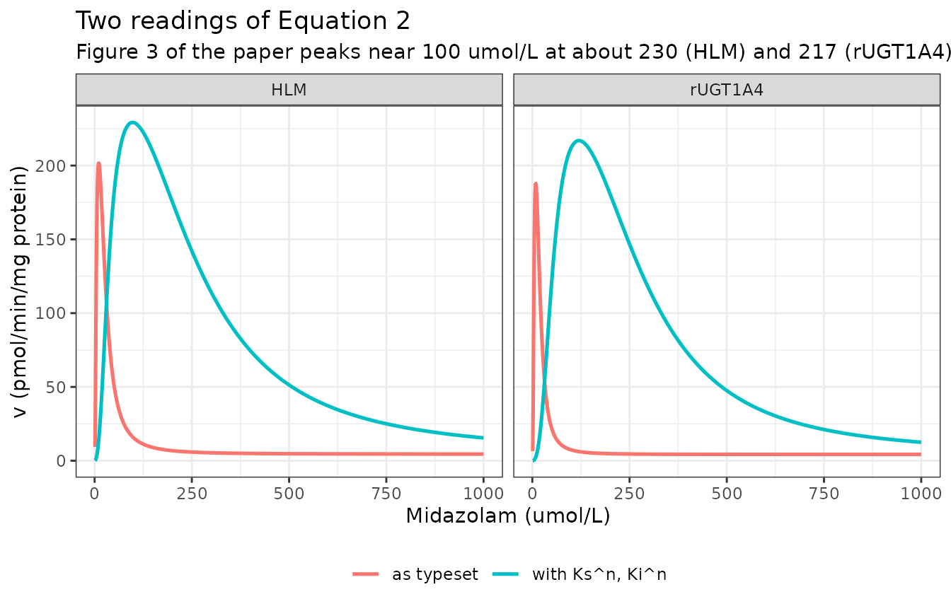
Source Figure 3 plots both fitted curves against midazolam concentration on a 0-1000 umol/L axis with the rate axis labelled every 20 units to 240. Two facts are readable off that axis without any digitisation: the maximum of each fitted curve lies to the left of the 200 umol/L tick, and it lies between the 220 and 240 rate labels. The reading with and satisfies both; the form as typeset puts the maximum an order of magnitude too far left.
peak <- function(f, p) {
  o <- optimize(function(s) do.call(f, c(list(s), as.list(p))), c(0.1, 1000), maximum = TRUE)
  c(S = o$maximum, v = o$objective)
}
pk <- bind_rows(lapply(names(pars), function(nm) {
  data.frame(system = nm,
             reading = c("as typeset", "with Ks^n, Ki^n"),
             rbind(peak(v_printed, pars[[nm]]), peak(v_hill, pars[[nm]])))
}))
knitr::kable(pk, digits = 1,
caption = "Location and height of the fitted maximum under each reading.")| system | reading | S | v |
|---|---|---|---|
| HLM | as typeset | 10.5 | 201.8 |
| HLM | with Ks^n, Ki^n | 97.6 | 229.2 |
| rUGT1A4 | as typeset | 8.7 | 188.0 |
| rUGT1A4 | with Ks^n, Ki^n | 120.0 | 216.9 |
# Bounds read off the printed axis of Figure 3, deliberately generous:
# the peak sits well inside the first 200 umol/L division and between the
# 220 and 240 rate labels. These are DETERMINISTIC quantities -- the models
# carry no random effects -- so a tight bound is correct here.
ok <- pk$reading == "with Ks^n, Ki^n"
stopifnot(
  all(pk$S[ok]  > 60  & pk$S[ok]  < 160),
  all(pk$v[ok]  > 205 & pk$v[ok]  < 245),
  # ... and the form as typeset is excluded by the same bounds, by a wide margin.
  all(pk$S[!ok] < 20)
)
(c) The printed form contradicts source Figure 4.
The inhibition experiment incubated midazolam “at a concentration
approximating to the Km” and reports uninhibited control
rates of 160.2, 154.2 and 150.0 pmol/mg/min for the ketoconazole,
itraconazole and trifluoperazine runs. The Abstract gives that
Km as 46 umol/L for HLM.
ctrl <- c(KTZ = 160.2, ITZ = 154.2, TFP = 150.0)   # Figure 4 legend
at_km <- c("as typeset"      = v_printed(46, 445, 46, 58, 18.3, 2.3),
           "with Ks^n, Ki^n" = v_hill(46, 445, 46, 58, 18.3, 2.3))
knitr::kable(
  data.frame(Reading = names(at_km),
             `Predicted rate at 46 umol/L` = round(at_km, 1),
             `vs Figure 4 controls (150.0-160.2)` =
               sprintf("%+.0f%% to %+.0f%%",
                       100 * (at_km / max(ctrl) - 1), 100 * (at_km / min(ctrl) - 1)),
             check.names = FALSE),
  row.names = FALSE,
  caption = "Predicted uninhibited rate at the reported Km against the Figure 4 controls."
)| Reading | Predicted rate at 46 umol/L | vs Figure 4 controls (150.0-160.2) |
|---|---|---|
| as typeset | 58.5 | -63% to -61% |
| with Ks^n, Ki^n | 170.0 | +6% to +13% |
stopifnot(
  # The Hill reading lands within 20% of the observed control window;
  # the form as typeset is low by a factor of about 2.6.
  abs(at_km[["with Ks^n, Ki^n"]] / mean(ctrl) - 1) < 0.20,
  at_km[["as typeset"]] / mean(ctrl) < 0.5
)
This is a defect in the typesetting of Equation 2, not a modelling
choice: the exponents on Ks and Ki were lost.
The model files reproduce the fit the paper actually shows.
Replicating Figure 3
The models are solved as the experiment was run – a 20 minute incubation at a fixed midazolam concentration – and the formation rate is read off at the end.
solve_curve <- function(mod, S, minutes = 20) {
  ev <- do.call(rbind, lapply(seq_along(S), function(i) {
    data.frame(id = i, time = c(0, minutes), amt = c(S[i], NA_real_),
               evid = c(1L, 0L), cmt = "midazolam")
  }))
  out <- rxode2::rxSolve(mod, ev, returnType = "data.frame")
  out <- out[out$time == minutes, ]
  out$S <- S[out$id]
  out
}

Sobs <- c(seq(1, 300, by = 1), seq(305, 1000, by = 5))
curve_hlm <- solve_curve(mod_hlm, Sobs)
#> Warning: multi-subject simulation without without 'omega'
curve_ugt <- solve_curve(mod_ugt, Sobs)
#> Warning: multi-subject simulation without without 'omega'
fig3 <- bind_rows(
  transform(curve_hlm, system = "HLM101"),
  transform(curve_ugt, system = "rUGT1A4")
)
ggplot(fig3, aes(S, Cc, colour = system)) +
  geom_line(linewidth = 0.9) +
  scale_x_continuous(breaks = seq(0, 1000, by = 200), limits = c(0, 1000)) +
  scale_y_continuous(breaks = seq(0, 240, by = 20), limits = c(0, 245)) +
  labs(x = "Midazolam (umol/L)", y = "V (pmol/min/mg)", colour = NULL,
       title = "Replicates Figure 3 of Hyland 2009",
       subtitle = "MDZG kinetics fitted to a two-site substrate-inhibition cooperative binding model") +
  theme_bw() + theme(legend.position = "bottom")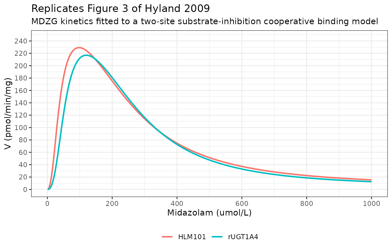
The published curves rise steeply to a maximum near 100-120 umol/L
and then decay across the rest of the axis, running close together
throughout with the HLM curve generally the upper of the two. That is
reproduced, with one caveat recorded below: between roughly 150 and 345
umol/L the implemented curves cross, putting rUGT1A4 up to 3% above HLM
where the published figure keeps HLM on top. The offset is a few
pmol/min/mg and is consistent with Table 4 reporting alpha
and n – the two parameters that most strongly set the curve
shape – to only two or three significant figures. It is recorded rather
than tuned away.
pk_hlm <- curve_hlm[which.max(curve_hlm$Cc), ]
pk_ugt <- curve_ugt[which.max(curve_ugt$Cc), ]
at <- function(d, s) d$Cc[which.min(abs(d$S - s))]

fig3_tab <- data.frame(
  Feature = c("HLM peak rate (pmol/min/mg)", "HLM peak location (umol/L)",
              "rUGT1A4 peak rate (pmol/min/mg)", "rUGT1A4 peak location (umol/L)",
              "HLM rate at 200 umol/L", "HLM rate at 400 umol/L",
              "HLM rate at 800 umol/L", "HLM vs rUGT1A4 at 800 umol/L"),
  Model = c(sprintf("%.1f", c(pk_hlm$Cc, pk_hlm$S, pk_ugt$Cc, pk_ugt$S,
                              at(curve_hlm, 200), at(curve_hlm, 400), at(curve_hlm, 800))),
            sprintf("%+.1f%%", 100 * (at(curve_hlm, 800) / at(curve_ugt, 800) - 1))),
  `Read from Figure 3` = c("between the 220 and 240 labels", "left of the 200 tick",
                           "between the 200 and 220 labels", "left of the 200 tick",
                           "just under 180", "between 60 and 90",
                           "between 10 and 30", "HLM above rUGT1A4 in the tail"),
  check.names = FALSE
)
knitr::kable(fig3_tab, caption = "Model against features readable off the printed axis of Figure 3.")| Feature | Model | Read from Figure 3 |
|---|---|---|
| HLM peak rate (pmol/min/mg) | 229.2 | between the 220 and 240 labels |
| HLM peak location (umol/L) | 98.0 | left of the 200 tick |
| rUGT1A4 peak rate (pmol/min/mg) | 216.9 | between the 200 and 220 labels |
| rUGT1A4 peak location (umol/L) | 120.0 | left of the 200 tick |
| HLM rate at 200 umol/L | 175.3 | just under 180 |
| HLM rate at 400 umol/L | 74.7 | between 60 and 90 |
| HLM rate at 800 umol/L | 22.4 | between 10 and 30 |
| HLM vs rUGT1A4 at 800 umol/L | +19.8% | HLM above rUGT1A4 in the tail |
stopifnot(
  pk_hlm$Cc > 220 & pk_hlm$Cc < 240,
  pk_ugt$Cc > 200 & pk_ugt$Cc < 220,
  pk_hlm$S  > 60  & pk_hlm$S  < 200,
  pk_ugt$S  > 60  & pk_ugt$S  < 200,
  at(curve_hlm, 200) > 160 & at(curve_hlm, 200) < 190,
  at(curve_hlm, 400) > 60  & at(curve_hlm, 400) < 90,
  at(curve_hlm, 800) > 10  & at(curve_hlm, 800) < 30,
  # HLM sits above rUGT1A4 in the tail, where the published gap is real
  # (13-20%). Deliberately NOT asserted at 200-300 umol/L: there the two
  # published curves are nearly coincident and the implemented pair cross,
  # so an ordering test would be a knife-edge on Table 4's rounding rather
  # than a check on the model. See the caveat above and the Errata.
  at(curve_hlm, 600) > at(curve_ugt, 600),
  at(curve_hlm, 800) > at(curve_ugt, 800)
)

# The published curves run close together across the descending limb; so do
# these. Bound the separation rather than its sign where the sign is not robust.
sep <- curve_hlm %>%
  select(S, hlm = Cc) %>%
  inner_join(select(curve_ugt, S, ugt = Cc), by = "S") %>%
  filter(S >= 150, S <= 800) %>%
  mutate(pct = 100 * (hlm / ugt - 1))
cat(sprintf("HLM vs rUGT1A4 over 150-800 umol/L: %.1f%% to %+.1f%%\n",
            min(sep$pct), max(sep$pct)))
#> HLM vs rUGT1A4 over 150-800 umol/L: -3.3% to +19.8%
stopifnot(min(sep$pct) > -6, max(sep$pct) < 25)
Replicating Figure 2 (Eadie-Hofstee)
Source Figure 2 plots v against v/[S]. A
Michaelis-Menten enzyme gives a straight line with slope
-Km; the published plots are hooked in both directions,
which is the diagnostic the authors used to reject Michaelis-Menten. The
model reproduces that shape, and the reason it is hooked rather than
straight is worth stating: the low-substrate limb bends because of the
Hill exponent (allosteric activation) and the high-substrate limb bends
back because of substrate inhibition.
eh <- fig3 %>% filter(S >= 10, S <= 800) %>% mutate(v_over_S = Cc / S)
ggplot(eh, aes(v_over_S, Cc, colour = system)) +
  geom_path(linewidth = 0.9) +
  labs(x = "v/[S]", y = "v (pmol/min/mg)", colour = NULL,
       title = "Replicates Figure 2 of Hyland 2009",
       subtitle = "Eadie-Hofstee plots over the studied 10-800 umol/L range") +
  theme_bw() + theme(legend.position = "bottom")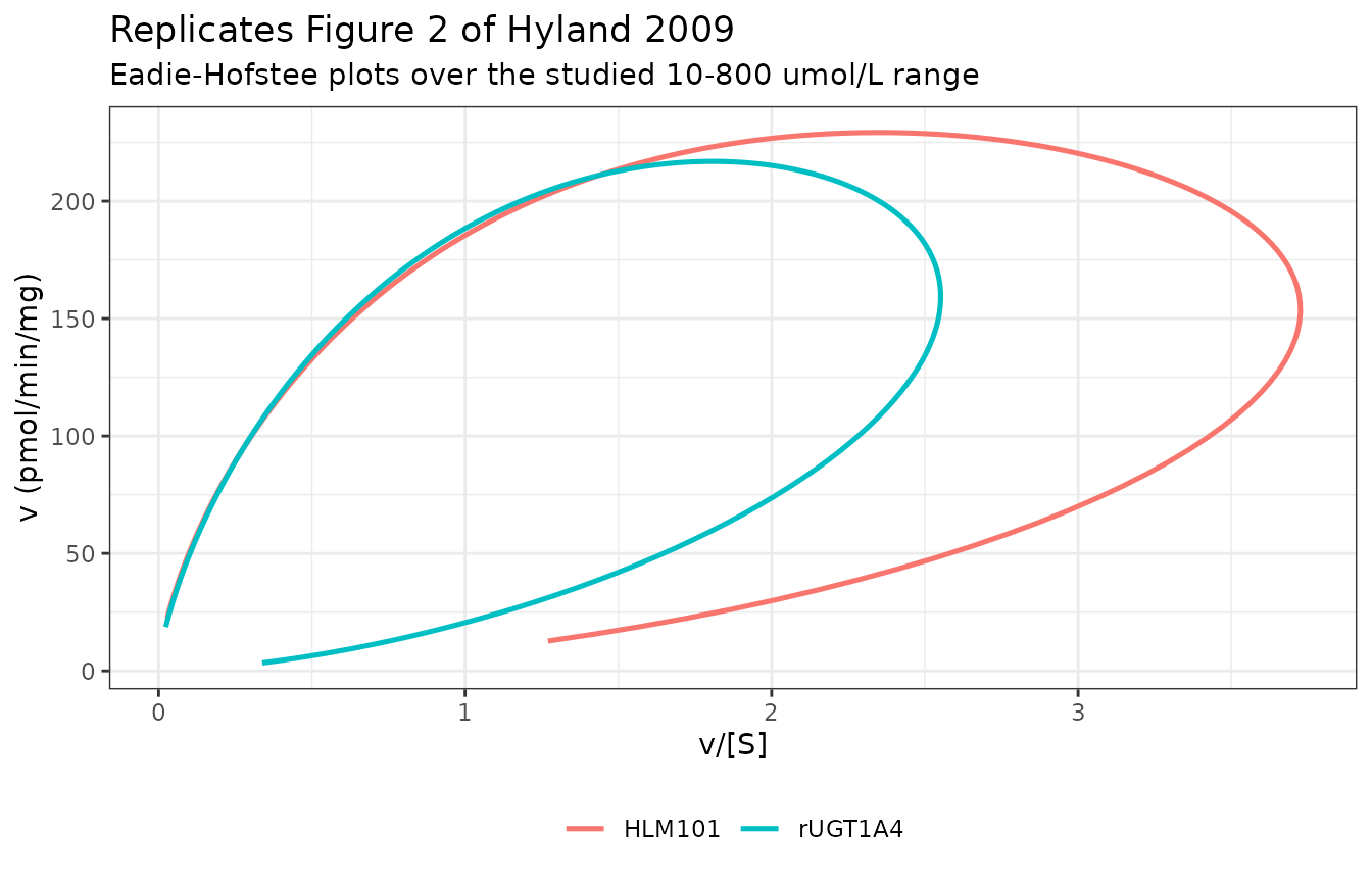
# The signature of the published plot: v/[S] is NOT monotone in [S] -- it rises
# with the allosteric limb and falls again -- so the curve doubles back. A
# Michaelis-Menten enzyme could not produce this.
hook <- eh %>% group_by(system) %>%
  summarise(max_v_over_S = max(v_over_S),
            v_over_S_at_lowest_S = v_over_S[which.min(S)],
            v_over_S_at_highest_S = v_over_S[which.max(S)], .groups = "drop")
knitr::kable(hook, digits = 3,
caption = "v/[S] doubles back: its maximum lies strictly inside the studied range.")| system | max_v_over_S | v_over_S_at_lowest_S | v_over_S_at_highest_S |
|---|---|---|---|
| HLM101 | 3.725 | 1.270 | 0.028 |
| rUGT1A4 | 2.551 | 0.338 | 0.023 |
Mechanistic checks
Product accumulation
The substrate is held constant, so the accumulated glucuronide must be exactly the rate times the incubation time. This is a pure numerical-identity check – both sides come from the same solve – so it is asserted tightly.
acc <- solve_curve(mod_hlm, c(10, 46, 100, 200, 400, 800), minutes = 20)
#> Warning: multi-subject simulation without without 'omega'
knitr::kable(
  data.frame(`Midazolam (umol/L)` = acc$S,
             `v (pmol/min/mg)` = round(acc$Cc, 2),
             `MDZG at 20 min (pmol/mg)` = round(acc$mdzg, 1),
             `v x 20 min` = round(acc$Cc * 20, 1),
             check.names = FALSE),
  row.names = FALSE,
  caption = "Accumulated MDZG equals the formation rate times the incubation time."
)| Midazolam (umol/L) | v (pmol/min/mg) | MDZG at 20 min (pmol/mg) | v x 20 min |
|---|---|---|---|
| 10 | 12.70 | 254.0 | 254.0 |
| 46 | 169.98 | 3399.6 | 3399.6 |
| 100 | 229.15 | 4583.0 | 4583.0 |
| 200 | 175.28 | 3505.5 | 3505.5 |
| 400 | 74.71 | 1494.3 | 1494.3 |
| 800 | 22.37 | 447.5 | 447.5 |
The initial-rate assumption
Holding the substrate constant is only legitimate if the incubation
consumes a small fraction of it. Over 20 minutes at 0.5 mg protein/mL
the amount turned over per mL is v * 20 * 0.5 pmol, so the
fraction of substrate consumed is
which is 1/100th of the Eadie-Hofstee ordinate. Source Figure 2
bounds v/[S] below 4 across the studied range, so at most
about 4% of the substrate is consumed – small enough for the
initial-rate treatment the published rate law assumes, but worth stating
rather than waving at.
protein_mg_per_mL <- 0.5    # Methods, 'MDZG kinetics': HLM at 0.5 mg protein/mL
minutes <- 20               # Methods, 'MDZG kinetics': 20 min incubation

# v [pmol/(min*mg)] * t [min] * p [mg/mL] = pmol/mL; 1 pmol/mL = 1e-3 umol/L.
depletion <- fig3 %>%
  filter(S >= 10, S <= 800) %>%
  mutate(pct_consumed = 100 * Cc * minutes * protein_mg_per_mL * 1e-3 / S)

worst <- depletion %>% slice_max(pct_consumed, n = 1)
shown <- depletion %>%
  filter(system == "HLM101", S %in% c(10, 46, 100, 400, 800)) %>%
  select(`Midazolam (umol/L)` = S, `v (pmol/min/mg)` = Cc,
         `Substrate consumed in 20 min (%)` = pct_consumed)
knitr::kable(shown, digits = c(0, 1, 2), row.names = FALSE,
caption = "Fraction of substrate consumed during the incubation (HLM).")| Midazolam (umol/L) | v (pmol/min/mg) | Substrate consumed in 20 min (%) |
|---|---|---|
| 10 | 12.7 | 1.27 |
| 46 | 170.0 | 3.70 |
| 100 | 229.2 | 2.29 |
| 400 | 74.7 | 0.19 |
| 800 | 22.4 | 0.03 |
cat(sprintf("Worst case over the studied range: %.2f%% consumed, at %.0f umol/L (%s)\n",
            worst$pct_consumed, worst$S, worst$system))
#> Worst case over the studied range: 3.73% consumed, at 41 umol/L (HLM101)

stopifnot(
  # Deterministic model, so this is a hard bound, not a quantile.
  max(depletion$pct_consumed) < 5,
  # Equivalently: max(v/[S]) < 4, which is exactly why Figure 2's x axis
  # runs to 4. The form as typeset would put v/[S] near 20 and could not
  # have been plotted on that axis at all.
  max(depletion$Cc / depletion$S) < 4
)
That last equivalence is a fourth check on the reading of Equation 2. Both panels of source Figure 2 use an Eadie-Hofstee axis running from 0 to 4, with the HLM points reaching roughly 3.8 and the rUGT1A4 points roughly 2.9.
eh_range <- bind_rows(
  data.frame(system = c("HLM101", "rUGT1A4"), reading = "as typeset",
             `max v/[S]` = c(max(v_printed(Sobs2 <- seq(10, 800, by = 0.25), 445, 46, 58, 18.3, 2.3) / Sobs2),
                             max(v_printed(Sobs2, 427, 64, 79, 14.9, 2.6) / Sobs2)),
             check.names = FALSE),
  data.frame(system = c("HLM101", "rUGT1A4"), reading = "with Ks^n, Ki^n",
             `max v/[S]` = c(max(v_hill(Sobs2, 445, 46, 58, 18.3, 2.3) / Sobs2),
                             max(v_hill(Sobs2, 427, 64, 79, 14.9, 2.6) / Sobs2)),
             check.names = FALSE)
)
eh_range$`fits the 0-4 axis of Figure 2` <- eh_range$`max v/[S]` < 4
knitr::kable(eh_range, digits = 2,
caption = "Maximum Eadie-Hofstee ordinate under each reading of Equation 2.")| system | reading | max v/[S] | fits the 0-4 axis of Figure 2 |
|---|---|---|---|
| HLM101 | as typeset | 20.16 | FALSE |
| rUGT1A4 | as typeset | 18.55 | FALSE |
| HLM101 | with Ks^n, Ki^n | 3.73 | TRUE |
| rUGT1A4 | with Ks^n, Ki^n | 2.55 | TRUE |
The high-substrate asymptote
As substrate saturates both sites, every term but the doubly-occupied
one drops out and the rate tends to Vmax * beta. That is
the mechanistic meaning of the fixed beta = 0.01: the
doubly-occupied enzyme still turns over, at 1% of the fully-saturated
rate. It is why the published curves decay toward a small non-zero value
rather than to zero.
asym <- data.frame(
  system = c("HLM101", "rUGT1A4"),
  `Vmax x beta` = c(445 * 0.01, 427 * 0.01),
  `v at 100000 umol/L` = c(v_hill(1e5, 445, 46, 58, 18.3, 2.3),
                           v_hill(1e5, 427, 64, 79, 14.9, 2.6)),
  check.names = FALSE
)
knitr::kable(asym, digits = 3, caption = "The rate law tends to Vmax * beta at saturating substrate.")| system | Vmax x beta | v at 100000 umol/L |
|---|---|---|
| HLM101 | 4.45 | 4.45 |
| rUGT1A4 | 4.27 | 4.27 |
In vivo urinary MDZG
The in vivo arm of the paper is descriptive mass-balance accounting rather than a fitted pharmacokinetic model, so it is not encoded in either model file. It is reproduced here because it is the paper’s headline result – the first demonstration that this pathway operates in people.
urine <- tibble::tribble(
  ~Subject, ~`3 mg oral (ug)`, ~`1 mg i.v. (ug)`,
  "3",  56.3, 40.7,
  "4",  21.0, 20.8,
  "5", 148.2, 59.8,
  "6",  59.2, 17.6,
  "10", 37.1, 26.5,
  "11", 35.3, 35.1,
  "Geometric mean", 48.8, 26.5,
  "SEM", 13.2, 5.7
)
knitr::kable(urine, caption = "Source Table 3: MDZG recovered in urine over 24 h in six healthy men (reproduced verbatim, including the i.v. summary row -- see below).")| Subject | 3 mg oral (ug) | 1 mg i.v. (ug) |
|---|---|---|
| 3 | 56.3 | 40.7 |
| 4 | 21.0 | 20.8 |
| 5 | 148.2 | 59.8 |
| 6 | 59.2 | 17.6 |
| 10 | 37.1 | 26.5 |
| 11 | 35.3 | 35.1 |
| Geometric mean | 48.8 | 26.5 |
| SEM | 13.2 | 5.7 |
The i.v. geometric mean printed in Table 3 is wrong. Recomputing it from the six tabulated subject values gives 30.6 ug, not 26.5 – and 30.6 is what the Results text (“an average of 30.7 +/- 5.7 ug”) and the Discussion (“49 ug and 31 ug”) both report. The printed 26.5 is subject 10’s own i.v. value, so it looks like a copy-down slip in the table. The oral column is self-consistent.
subj <- urine[1:6, ]
gm <- function(x) exp(mean(log(x)))
knitr::kable(
  data.frame(
    Route = c("3 mg oral", "1 mg i.v."),
    `Table 3 prints` = c(48.8, 26.5),
    `Recomputed geometric mean` = round(c(gm(subj$`3 mg oral (ug)`), gm(subj$`1 mg i.v. (ug)`)), 1),
    `Results text` = c("48.8", "30.7"),
    check.names = FALSE
  ),
  row.names = FALSE,
  caption = "The oral summary reproduces; the i.v. one does not."
)| Route | Table 3 prints | Recomputed geometric mean | Results text |
|---|---|---|---|
| 3 mg oral | 48.8 | 48.8 | 48.8 |
| 1 mg i.v. | 26.5 | 30.6 | 30.7 |
stopifnot(
  abs(gm(subj$`3 mg oral (ug)`) - 48.8) < 0.2,   # oral row is self-consistent
  abs(gm(subj$`1 mg i.v. (ug)`) - 30.7) < 0.2,   # i.v. matches the TEXT, not the table
  abs(gm(subj$`1 mg i.v. (ug)`) - 26.5) > 3      # ... and is genuinely far from the printed value
)
Nothing in either model file depends on this row; it is recorded because the source trace has to be honest about which printed numbers reproduce.
MDZG accounted for roughly 1-2% of the administered dose on a molar basis, with more than 70% of it excreted in the first 12 h under both routes. Between-subject variability was about sevenfold after oral dosing and 3.4-fold after intravenous dosing – the same sevenfold spread the authors saw across a 56-donor bank of liver microsomes.
Assumptions and deviations
- Equation 2 is implemented with and , not as typeset. The form printed in the paper is dimensionally inconsistent, reproduces neither Figure 3 nor the Figure 4 control rates, and disagrees with the Shou et al. model the Methods cite as its source. All three checks are run above as render-time gates. This is the single deviation from the printed source, and it is a correction of the typesetting, not of the model. Both model files carry the same reasoning inline.
-
Known deviation: the two curves cross between about 150 and
345 umol/L. Source Figure 3 keeps the HLM curve above the
rUGT1A4 curve across the whole descending limb. The implemented pair
cross twice, with rUGT1A4 up to 3.2% (about 5 pmol/min/mg) above HLM in
that window; outside it the published ordering is reproduced, reaching a
20% gap by 800 umol/L. Table 4 reports
alpha(18.3 vs 14.9) andn(2.3 vs 2.6) to two or three significant figures, and those two parameters dominate the curve shape, so a sub-5% vertical offset between two nearly-coincident curves is within the published precision. No parameter was adjusted to remove it; the ordering gate is asserted only in the tail, where the published separation is large enough to be meaningful. - The rate law is written multiplied through by . Algebraically identical to the printed ratio, but finite at , where the printed form evaluates . This is also how Shou et al. write the model.
-
No residual error. The paper reports fit quality
only as
(0.962 for HLM, 0.986 for rUGT1A4) and gives no residual standard
deviation, so
addSdisfixed(0)rather than invented. Both models are deterministic: they carry no random effects at all, which is why the assertions above are tight rather than quantile-based. - No inter-individual variability. The HLM preparation is a pool and the recombinant enzyme is a single expressed protein; neither fit has a subject dimension. The paper separately notes a sevenfold range in MDZG formation across a 56-donor microsome bank, but reports no variance component for it.
-
The ketoconazole, itraconazole and trifluoperazine effects
are not encoded. Source Figure 4 reports IC50 values of 150 +/-
6 umol/L (ketoconazole) and 308 +/- 14 umol/L (itraconazole), and a
maximal trifluoperazine activation of 138% at 60 umol/L. No inhibition
equation, Hill slope or mechanism is published for any of the three. The
fitted sigmoids in Figure 4 are visibly steeper than a slope-1 curve, so
encoding them with an assumed slope of 1 would misrepresent the
published data, and inventing a slope is not permitted. The values are
recorded in each model file’s
population$notesinstead. The authors’ own conclusion is that this inhibition is weak enough to be irrelevant in vivo. - The Simcyp simulation is out of scope. The Discussion reports a population-ADME simulation (Simcyp v8.1, 10 populations of 10 individuals, 3 mg oral midazolam) in which UGT1A4 contributes 2.9% of hepatic intrinsic clearance uninhibited and 19% with 400 mg ketoconazole co-administered. That simulation runs on “the default MDZ profile provided by Simcyp”, a proprietary platform parameter set that is not in the paper or any supplement. Platform PBPK models are out of scope for this library and none of those parameters may be substituted from elsewhere, so only the enzyme-kinetic layer the paper itself reports is extracted.
- PKNCA is not used. There is no dose, no absorption-distribution- elimination profile and no concentration-time curve to integrate; this is an enzyme-kinetic model, so the validation follows the mechanistic pattern (dimensional analysis, mass balance, limiting behaviour, figure replication) rather than non-compartmental analysis.
-
“Km” versus
Ks. The Abstract and Discussion call the productive-binding dissociation constantKm(46 and 64 umol/L); Table 4 and Equation 2 call itKs. They are the same quantity. The model files uselks, matching the equation. -
No parameter was digitised. Every value in both
ini()blocks comes from Table 4 or from the Results text. Figures 3 and 4 are used only to check the implementation, never to source a value.