Morphine, M3G and M6G (Oosten 2017) • nlmixr2lib

Model and source

Citation: Oosten AW, Abrantes JA, Jonsson S, Matic M, van Schaik RHN, de Bruijn P, van der Rijt CCD, Mathijssen RHJ. A Prospective Population Pharmacokinetic Study on Morphine Metabolism in Cancer Patients. Clin Pharmacokinet. 2017;56(6):649-659 (published online 5 November 2016). doi:10.1007/s40262-016-0471-7.
Description: Joint parent-metabolite population PK model for morphine and its two glucuronide metabolites (M3G, M6G) in 49 adult cancer patients treated for nociceptive cancer pain (Oosten 2017). Morphine: one-compartment disposition with three parallel first-order absorption routes (subcutaneous, oral immediate release, oral extended release with a lag time); the subcutaneous route is assumed completely bioavailable and the oral routes carry an extensive first pass. The oral first pass is a four-way partition of the absorbed dose - unchanged morphine, M3G, M6G and a residual lost fraction - parameterised as odds against the unchanged route, which is what makes oral bioavailability (0.372) and the first-pass metabolite fractions (0.355 for M3G, 0.0631 for M6G) sum to at most one by construction. M3G and M6G are each one-compartment models fed both by this oral first pass and by fixed-fraction transformation of systemic morphine clearance (0.57 to M3G, 0.10 to M6G, both fixed from literature); the two metabolites share a single estimated clearance and volume and differ only in how much of them is formed. Allometric body weight with theory-based exponents is applied a priori to every disposition parameter of every entity, and metabolite clearance rises linearly with estimated glomerular filtration rate up to a plateau at 90 mL/min/1.73 m^2. All amounts are nmol of the free base and all concentrations nmol/L, so the 1:1 molar conversion of morphine to each glucuronide needs no molecular-weight factor.
Article: https://doi.org/10.1007/s40262-016-0471-7
Supplement (SIR procedure, observation plots): retrieved from EuropePMC PMC5488155 supplementary files; it contains no parameter values beyond the main text.

Oosten 2017 fitted morphine together with its two glucuronide metabolites in one NONMEM run, so the whole paper is a single coupled model and is packaged as a single model file.

Population

410 plasma samples from 49 adults admitted to the Erasmus MC Cancer Institute (Rotterdam) with moderate to severe nociceptive cancer-related pain, enrolled February 2010 to March 2014 (Dutch Trial Register NTR4369). Median age 60 years (38-80), median weight 83 kg (53-140), 45% female, 90% Caucasian; 89% had distant metastases and the median WHO performance status was 2. Median baseline creatinine was 72 umol/L (25-190) and median eGFR 81 mL/min/1.73 m^2, with values above 90 truncated at 90 and seven patients between 33 and 57 (Oosten 2017 Table 2).

During sampling 57% of patients received subcutaneous morphine only, 24% oral extended-release plus immediate-release, 12% oral immediate-release only, and 6% both oral and subcutaneous consecutively. Median doses were 2 mg/h subcutaneously (0.6-14 mg/h), 40 mg twice daily orally as extended release (10-150 mg) and 10 mg as immediate release (5-60 mg).

The same information is available programmatically via readModelDb("Oosten_2017_morphine")()$population.

Model structure

Morphine follows one-compartment disposition fed by three parallel first-order absorption routes. The subcutaneous route is assumed completely bioavailable; both oral routes pass through an extensive first pass that splits the absorbed dose four ways at a single point – unchanged morphine into the central compartment, M3G and M6G straight into their own compartments, and a residual fraction lost. M3G and M6G are each one-compartment models that additionally receive fixed fractions of systemic morphine clearance. They share a single estimated clearance and a single estimated volume and differ only in how much of each is formed, and in their independent random effects.

Table 3 footnote b parameterises the first-pass split as odds against the route delivering unchanged morphine:

F_oral   = 1      / (1 + theta1 + theta2 + theta3)
F1p,M3G  = theta2 / (1 + theta1 + theta2 + theta3)
F1p,M6G  = theta1 / (1 + theta1 + theta2 + theta3)

which is what makes the shares sum to at most one by construction – the constraint the Methods describe. The model file keeps the thetas primary (as lfprat_m3g, lfprat_m6g, lfprat_other) because the published random effects sit on theta1 and theta3 and propagate non-linearly to all four shares through the shared denominator; an eta placed on a derived fraction could not reproduce that structure.

All amounts are nmol of morphine free base and all concentrations are nmol/L (Methods 2.4), so the 1:1 molar conversion of morphine into each glucuronide needs no molecular-weight factor.

Source trace

Every ini() entry in inst/modeldb/specificDrugs/Oosten_2017_morphine.R carries an in-file comment naming its origin. They are collected here for review.

Equation / parameter	Value	Source location
`ltlag_er`	0.25 h (fixed)	Table 3, `t lag, ER`
`lka_sc`	3.96 /h (fixed)	Table 3, `k a, SC`; literature value, refs 27-28
`lka_oral_ir`	6.00 /h (fixed)	Table 3, `k a, IR`; literature value, refs 27-28
`lka_oral_er`	0.221 /h	Table 3, `k a, ER` (RSE 17.7%, CI 0.155-0.306)
`lfprat_m3g`	0.953	Table 3, `theta 2` (RSE 8.95%, CI 0.796-1.14)
`lfprat_m6g`	0.170	Table 3, `theta 1` (RSE 10.4%, CI 0.136-0.206)
`lfprat_other`	0.565	Table 3, `theta 3` (RSE 30.3%, CI 0.310-1.01)
derived `F_oral` = 1/(1+t1+t2+t3)	0.372	Table 3 footnote b and row `F oral`
derived `F1p,M3G` = t2/(1+t1+t2+t3)	0.355	Table 3 footnote b and row `F 1p, M3G`
derived `F1p,M6G` = t1/(1+t1+t2+t3)	0.0631	Table 3 footnote b and row `F 1p, M6G`
`lcl`	91.9 L/h	Table 3, `CL 70kg` (RSE 3.91%, CI 85.8-99.9)
`lvc`	278 L	Table 3, `V 70kg` (RSE 12.3%, CI 221-351)
`e_wt_cl`, `e_wt_cl_m3g`, `e_wt_cl_m6g`	0.75 (fixed)	Table 3 footnote c
`e_wt_vc`, `e_wt_vc_m3g`, `e_wt_vc_m6g`	1 (fixed)	Table 3 footnote c
`fm_m3g`	0.57 (fixed)	Results 3.2 prose; see Errata (Table 3 prints 0.573)
`fm_m6g`	0.10 (fixed)	Results 3.2 prose; see Errata (Table 3 prints 0.104)
`lcl_m3g`, `lcl_m6g`	4.71 L/h	Table 3, `CL met, 70kg` (RSE 5.24%); one estimate common to both
`lvc_m3g`, `lvc_m6g`	25.8 L	Table 3, `V met, 70kg` (RSE 6.12%); one estimate common to both
`e_crcl_cl_m3g`, `e_crcl_cl_m6g`	0.0128	Table 3, `eGFR on CL met, 70kg` (RSE 12.9%)
eGFR truncation at 90	n/a	Methods 2 (“values > 90 … were truncated”) and Results 3.2
`etalka`	71.0% CV	Table 3 IIV, `k a, all`
`etalcl`	22.2% CV	Table 3 IIV, `CL 70kg`
`etalvc`	74.7% CV	Table 3 IIV, `V 70kg`
`etalcl_m3g` / `etalcl_m6g` block	36.2% / 36.8% CV, rho 0.912	Table 3 IIV and `Correlation CL M3G - CL M6G`, footnote e
`etalvc_m3g`, `etalvc_m6g`	24.7%, 24.3% CV	Table 3 IIV, `V M3G` / `V M6G`
`etalfprat_m6g`, `etalfprat_other`	15.0%, 98.2% CV	Table 3 IIV, `theta 1` / `theta 3`
`propSd`, `propSd_m3g`, `propSd_m6g`	0.286, 0.200, 0.239	Table 3 residual variability, footnote a
ODE topology (three depots, first-pass arrows, `CL * Fm` arms)	n/a	Figure 1

mod <- readModelDb("Oosten_2017_morphine")
ui <- rxode2::rxode(mod)

# Doses were handled as free base in molar units (Methods 2.4). The salts the
# study used, with the molecular weights the paper states:
#   parenteral: morphine hydrochloride-3-water, 375.84 mg/mmol, 1 morphine/mol
#   oral:       morphine 5-sulphate-water,      758.83 mg/mmol, 2 morphine/mol
nmol_sc <- function(mg) mg / 375.84 * 1e6
nmol_oral <- function(mg) mg / 758.83 * 2 * 1e6

# This model declares three endpoints (Cc, Cc_m3g, Cc_m6g), so rxode2 assigns
# their slots AFTER the six ODE states. Observation rows must therefore carry
# cmt = "Cc" (slot 7), not cmt = "central" (slot 4), which errors with
# "'dvid'->'cmt' ... on a undefined compartment". rxSolve still returns all
# three endpoint columns from a single endpoint's observation rows.
ui$predDf[, c("cond", "var", "dvid", "cmt")]
#>     cond    var dvid cmt
#> 1     Cc     Cc    1   7
#> 2 Cc_m3g Cc_m3g    2   8
#> 3 Cc_m6g Cc_m6g    3   9

Typical-value replication of the published derived quantities

The first-pass fractions are not estimated directly; they are functions of the three odds parameters. Recovering the published values is the cheapest check that the partition is transcribed correctly.

typical_solve <- function(cmt_dose, amt, wt = 70, egfr = 81,
                          times = c(seq(0, 24, by = 0.02), seq(24.1, 96, by = 0.1)),
                          params = NULL) {
  ev <- rxode2::et(amt = amt, cmt = cmt_dose, time = 0) |>
    rxode2::et(times, cmt = "Cc")
  d <- as.data.frame(ev)
  d$WT <- wt
  d$CRCL <- egfr
  args <- list(
    object = mod, events = d, omega = NA, returnType = "data.frame",
    # rxode2's automatic ODE -> linCmt conversion can corrupt the dvid mapping
    # for multi-output models; disable it (see known-vignette-failure-patterns
    # pattern 5b).
    useLinCmt = FALSE
  )
  if (!is.null(params)) args$params <- params
  do.call(rxode2::rxSolve, args)
}

ref <- typical_solve("depot3", nmol_oral(40))

derived <- tibble::tibble(
  Quantity = c("F_oral", "F1p,M3G", "F1p,M6G", "residual lost fraction"),
  Simulated = c(ref$fdepot[1], ref$f1p_m3g[1], ref$f1p_m6g[1],
                1 - ref$fdepot[1] - ref$f1p_m3g[1] - ref$f1p_m6g[1]),
  Published = c(0.372, 0.355, 0.0631, NA_real_),
  `Table 3 row` = c("F oral", "F 1p, M3G", "F 1p, M6G", "not reported")
)
knitr::kable(derived, digits = 4,
             caption = "Derived first-pass fractions vs Oosten 2017 Table 3.")

Derived first-pass fractions vs Oosten 2017 Table 3.
Quantity	Simulated	Published	Table 3 row
F_oral	0.3720	0.3720	F oral
F1p,M3G	0.3545	0.3550	F 1p, M3G
F1p,M6G	0.0632	0.0631	F 1p, M6G
residual lost fraction	0.2102	NA	not reported


# Deterministic quantities, so the tolerance is set by rounding alone. The
# model recomputes each fraction from the ROUNDED thetas Table 3 prints, while
# the paper printed each fraction from its own unrounded estimates, so the two
# can disagree in the last digit: F1p,M6G is 0.170 / 2.688 = 0.06324 here
# against a printed 0.0631 (0.23%), and theta1 = 0.1696 would reproduce the
# printed value exactly. 0.5% covers that and still goes red on any real
# transcription error, which would move these by whole per cent.
stopifnot(
  abs(ref$fdepot[1] / 0.372 - 1) < 0.005,
  abs(ref$f1p_m3g[1] / 0.355 - 1) < 0.005,
  abs(ref$f1p_m6g[1] / 0.0631 - 1) < 0.005,
  # The four shares sum to exactly one by construction.
  abs(ref$fdepot[1] + ref$f1p_m3g[1] + ref$f1p_m6g[1] +
        exp(ui$theta[["lfprat_other"]]) / (1 + exp(ui$theta[["lfprat_m6g"]]) +
          exp(ui$theta[["lfprat_m3g"]]) + exp(ui$theta[["lfprat_other"]])) - 1) < 1e-12
)

Covariate model

cl_met <- function(wt, egfr) {
  s <- typical_solve("depot", nmol_sc(1), wt = wt, egfr = egfr, times = c(0, 1))
  s$cl_m3g[1]
}

# Abstract: metabolite clearance "increased 0.602 L/h with every increase in
# eGFR of 10 mL/min/1.73 m^2".
slope_per_10 <- cl_met(70, 90) - cl_met(70, 80)

# Results 3.2: "up to an eGFR of 90 mL/min/1.73 m^2, above which clearance was
# constant".
plateau_gap <- cl_met(70, 120) - cl_met(70, 90)

# Table 3 footnotes c and d: theory-based allometric exponents.
allom_cl <- cl_met(140, 81) / cl_met(70, 81)

tibble::tibble(
  Check = c("dCLmet per 10 mL/min/1.73 m^2 eGFR (L/h)",
            "CLmet(eGFR 120) - CLmet(eGFR 90) (L/h)",
            "CLmet(140 kg) / CLmet(70 kg)"),
  Simulated = c(slope_per_10, plateau_gap, allom_cl),
  Published = c(0.602, 0, 2^0.75)
) |>
  knitr::kable(digits = 4, caption = "Covariate-model checks.")

Covariate-model checks.
Check	Simulated	Published
dCLmet per 10 mL/min/1.73 m^2 eGFR (L/h)	0.6029	0.6020
CLmet(eGFR 120) - CLmet(eGFR 90) (L/h)	0.0000	0.0000
CLmet(140 kg) / CLmet(70 kg)	1.6818	1.6818


stopifnot(
  abs(slope_per_10 - 0.602) < 5e-3,
  plateau_gap == 0,
  abs(allom_cl - 2^0.75) < 1e-9
)

plateau_gap == 0 is an exact-equality assertion on a deterministic quantity (no cohort, no random draw): above 90 mL/min/1.73 m^2 the model substitutes the truncated value, so the two clearances are the same floating-point number.

Reproducing the published AUC ratios

Oosten 2017 reports no absolute NCA values, so there is nothing to feed nlmixr2lib::ncaComparisonTable(). What it does report – the paper’s headline result – is six mean AUC molar ratios for a typical patient (70 kg, eGFR 81 mL/min/1.73 m^2) after oral versus subcutaneous morphine (Results 3.2). Those ratios are a strong structural gate: the subcutaneous ones contain no first-pass term at all, so they pin the systemic metabolic fractions directly, while the oral ones additionally exercise the whole first-pass partition.

AUC is computed with PKNCA, over a window long enough that auclast is indistinguishable from aucinf (morphine t1/2 = ln2 * 278 / 91.9 = 2.1 h, metabolite t1/2 = ln2 * 25.8 / 4.71 = 3.8 h, window 96 h).

auc_of <- function(s, col) {
  PKNCA::pk.calc.auc.last(conc = s[[col]], time = s$time)
}

ratio_row <- function(label, s) {
  a <- auc_of(s, "Cc")
  tibble::tibble(
    Route = label,
    `M3G:morphine` = auc_of(s, "Cc_m3g") / a,
    `M6G:morphine` = auc_of(s, "Cc_m6g") / a,
    `M3G:M6G` = auc_of(s, "Cc_m3g") / auc_of(s, "Cc_m6g")
  )
}

sc_typ <- typical_solve("depot", nmol_sc(10))
er_typ <- typical_solve("depot3", nmol_oral(40))
ir_typ <- typical_solve("depot2", nmol_oral(10))

sim_ratios <- dplyr::bind_rows(
  ratio_row("Subcutaneous", sc_typ),
  ratio_row("Oral extended release", er_typ),
  ratio_row("Oral immediate release", ir_typ)
)

published_ratios <- tibble::tribble(
  ~Route, ~`M3G:morphine`, ~`M6G:morphine`, ~`M3G:M6G`,
  "Subcutaneous", 11.1, 1.95, 5.70,
  "Oral extended release", 29.7, 5.26, 5.65,
  "Oral immediate release", 29.7, 5.26, 5.65
)

cmp <- dplyr::bind_rows(
  sim_ratios |> dplyr::mutate(Source = "Simulated"),
  published_ratios |> dplyr::mutate(Source = "Oosten 2017 Results 3.2")
) |>
  dplyr::relocate(Source, .after = Route) |>
  dplyr::arrange(Route, Source)

knitr::kable(cmp, digits = 3,
             caption = paste("Mean AUC molar ratios for a typical patient",
                             "(70 kg, eGFR 81 mL/min/1.73 m^2).",
                             "Oosten 2017 reports one oral column; the model",
                             "predicts the same ratios for both oral",
                             "formulations, because an AUC ratio is invariant",
                             "to the absorption rate constant."))

Mean AUC molar ratios for a typical patient (70 kg, eGFR 81 mL/min/1.73 m^2). Oosten 2017 reports one oral column; the model predicts the same ratios for both oral formulations, because an AUC ratio is invariant to the absorption rate constant.
Route	Source	M3G:morphine	M6G:morphine	M3G:M6G
Oral extended release	Oosten 2017 Results 3.2	29.700	5.260	5.650
Oral extended release	Simulated	29.716	5.268	5.641
Oral immediate release	Oosten 2017 Results 3.2	29.700	5.260	5.650
Oral immediate release	Simulated	29.718	5.268	5.641
Subcutaneous	Oosten 2017 Results 3.2	11.100	1.950	5.700
Subcutaneous	Simulated	11.122	1.951	5.700


pct <- function(sim, pub) 100 * abs(sim - pub) / pub
dev <- dplyr::inner_join(sim_ratios, published_ratios, by = "Route",
                         suffix = c("_sim", "_pub")) |>
  dplyr::mutate(
    d_m3g_m = pct(`M3G:morphine_sim`, `M3G:morphine_pub`),
    d_m6g_m = pct(`M6G:morphine_sim`, `M6G:morphine_pub`),
    d_m3g_m6g = pct(`M3G:M6G_sim`, `M3G:M6G_pub`)
  )
print(dev[, c("Route", "d_m3g_m", "d_m6g_m", "d_m3g_m6g")])
#> # A tibble: 3 × 4
#>   Route                  d_m3g_m d_m6g_m d_m3g_m6g
#>   <chr>                    <dbl>   <dbl>     <dbl>
#> 1 Subcutaneous            0.200   0.0645  1.48e-12
#> 2 Oral extended release   0.0547  0.155   1.64e- 1
#> 3 Oral immediate release  0.0594  0.160   1.64e- 1

# Deterministic typical-value quantities, so a tight bound is correct here (see
# known-vignette-failure-patterns pattern 11 vs 12). Realised maximum is 0.21%,
# from rounding the published ratios to three significant figures. The bound
# can still go red: encoding the Table 3 metabolic fractions 0.573 / 0.104
# instead of the Results-text 0.57 / 0.10 moves the subcutaneous M6G:morphine
# ratio from 1.95 to 2.03, a 4.1% deviation (see Errata).
stopifnot(max(dev$d_m3g_m, dev$d_m6g_m, dev$d_m3g_m6g) < 1)

Mass-balance gates

An AUC ratio is blind to how the dose was split between input paths, so it is paired here with per-path recovery gates. Solving each route on its own and recovering the dose from CL * AUC is what discriminates a mis-transcribed bioavailability or first-pass fraction.

th <- ui$theta
fdep <- ref$fdepot[1]
f3 <- ref$f1p_m3g[1]
f6 <- ref$f1p_m6g[1]
fm3 <- 0.57
fm6 <- 0.10
CL <- 91.9
CLMET <- 4.71

balance <- tibble::tribble(
  ~Route, ~Entity, ~Recovered, ~Expected,
  "Subcutaneous", "morphine", CL * auc_of(sc_typ, "Cc"), nmol_sc(10),
  "Subcutaneous", "M3G", CLMET * auc_of(sc_typ, "Cc_m3g"), nmol_sc(10) * fm3,
  "Subcutaneous", "M6G", CLMET * auc_of(sc_typ, "Cc_m6g"), nmol_sc(10) * fm6,
  "Oral ER", "morphine", CL * auc_of(er_typ, "Cc"), nmol_oral(40) * fdep,
  "Oral ER", "M3G", CLMET * auc_of(er_typ, "Cc_m3g"),
    nmol_oral(40) * (f3 + fdep * fm3),
  "Oral ER", "M6G", CLMET * auc_of(er_typ, "Cc_m6g"),
    nmol_oral(40) * (f6 + fdep * fm6),
  "Oral IR", "morphine", CL * auc_of(ir_typ, "Cc"), nmol_oral(10) * fdep,
  "Oral IR", "M3G", CLMET * auc_of(ir_typ, "Cc_m3g"),
    nmol_oral(10) * (f3 + fdep * fm3),
  "Oral IR", "M6G", CLMET * auc_of(ir_typ, "Cc_m6g"),
    nmol_oral(10) * (f6 + fdep * fm6)
) |>
  dplyr::mutate(`Error (%)` = 100 * (Recovered - Expected) / Expected)

knitr::kable(balance, digits = c(0, 0, 1, 1, 4),
             caption = paste("Amount balance (nmol): CL * AUC recovered from",
                             "the solve versus the amount the model should",
                             "deliver down each path."))

Amount balance (nmol): CL * AUC recovered from the solve versus the amount the model should deliver down each path.
Route	Entity	Recovered	Expected	Error (%)
Subcutaneous	morphine	26605.8	26607.1	-0.0046
Subcutaneous	M3G	15166.0	15166.0	0.0000
Subcutaneous	M6G	2660.7	2660.7	0.0000
Oral ER	morphine	39220.8	39220.8	0.0001
Oral ER	M3G	59733.2	59733.2	0.0000
Oral ER	M6G	10589.6	10589.6	0.0000
Oral IR	morphine	9804.5	9805.2	-0.0069
Oral IR	M3G	14933.0	14933.3	-0.0023
Oral IR	M6G	2647.3	2647.4	-0.0024


# Pure numerical (trapezoid + truncation) error between two sides computed from
# the same parameters, so a tight absolute bound is correct.
stopifnot(max(abs(balance$`Error (%)`)) < 0.05)

The subcutaneous route carries no first pass

# Drive the first-pass M3G odds to ~0 and re-solve the identical event tables.
# The oral M3G exposure must fall substantially; the subcutaneous one must not
# move at all. This is the check that a silently dropped first-pass arm (or a
# partition applied to the wrong depot) cannot survive.
kill <- c(lfprat_m3g = log(1e-9))
er_nofp <- typical_solve("depot3", nmol_oral(40), params = kill)
sc_nofp <- typical_solve("depot", nmol_sc(10), params = kill)

drop_oral <- 1 - auc_of(er_nofp, "Cc_m3g") / auc_of(er_typ, "Cc_m3g")
drop_sc <- 1 - auc_of(sc_nofp, "Cc_m3g") / auc_of(sc_typ, "Cc_m3g")
c(oral_M3G_AUC_drop = drop_oral, sc_M3G_AUC_drop = drop_sc)
#> oral_M3G_AUC_drop   sc_M3G_AUC_drop 
#>         0.4201649         0.0000000

stopifnot(
  # Deterministic and closed-form. Setting theta2 to 0 removes the first-pass
  # M3G route AND shrinks the odds denominator from 2.688 to 1.735, so oral
  # bioavailability rises from 0.372 to 0.576 and part of the lost M3G returns
  # via the systemic route. Expected oral M3G exposure ratio is therefore
  # (0.576 * 0.57) / (0.3545 + 0.372 * 0.57) = 0.580, i.e. a 42.0% drop.
  drop_oral > 0.35, drop_oral < 0.50,
  # The subcutaneous route never touches the first-pass partition.
  abs(drop_sc) < 1e-9,
  # Subcutaneous M3G:M6G is exactly fm_m3g / fm_m6g, with no first-pass term.
  abs(auc_of(sc_typ, "Cc_m3g") / auc_of(sc_typ, "Cc_m6g") - fm3 / fm6) < 1e-3
)

Virtual cohort

Original observed data are not publicly available. The cohort below approximates the Table 2 demographics: weight log-normal about the 83 kg median and clipped to the published 53-140 kg range, eGFR normal about 81 and clipped to the published 33-90 range (values above 90 were truncated by the authors).

# `set.seed()` seeds R's RNG, which is what draws the covariates below. It does
# NOT seed rxode2's simulation RNG, whose streams are partitioned per solver
# thread -- so the eta draws differ between a 16-thread workstation and a
# 2-core CI runner and no seed can make them agree. Every assertion on a
# cohort-derived quantity below is therefore written as a robust
# median/quantile statement, never as a sign, an exact value or a bound taken
# from one run.
set.seed(20170605)

n_per_arm <- 150L

make_cohort <- function(n, admin_arm, cmt_dose, amt, id_offset = 0L) {
  subj <- tibble::tibble(
    id = id_offset + seq_len(n),
    WT = pmin(pmax(stats::rlnorm(n, log(83), 0.28), 53), 140),
    CRCL = pmin(pmax(stats::rnorm(n, 81, 18), 33), 90),
    admin_arm = admin_arm
  )
  # 48 h is 15-23 morphine half-lives and ~13 metabolite half-lives for a
  # typical subject, so auclast is within a rounding error of aucinf while the
  # tail stays well clear of the solver noise floor that a 96 h window reaches
  # for the fastest-clearing subjects (pattern 11 of
  # known-vignette-failure-patterns).
  times <- c(seq(0, 12, by = 0.1), seq(12.5, 24, by = 0.5), seq(25, 48, by = 1))
  doses <- subj |>
    dplyr::mutate(time = 0, amt = amt, evid = 1L, cmt = cmt_dose)
  obs <- subj |>
    tidyr::crossing(time = times) |>
    dplyr::mutate(amt = NA_real_, evid = 0L, cmt = "Cc")
  dplyr::bind_rows(doses, obs) |>
    dplyr::arrange(id, time, dplyr::desc(evid))
}

events <- dplyr::bind_rows(
  make_cohort(n_per_arm, "Subcutaneous", "depot", nmol_sc(10), id_offset = 0L),
  make_cohort(n_per_arm, "Oral extended release", "depot3", nmol_oral(40),
              id_offset = 1000L),
  make_cohort(n_per_arm, "Oral immediate release", "depot2", nmol_oral(10),
              id_offset = 2000L)
)
stopifnot(!anyDuplicated(unique(events[, c("id", "time", "evid")])))

sim <- rxode2::rxSolve(
  mod,
  events = events,
  keep = c("admin_arm"),
  useLinCmt = FALSE
) |>
  as.data.frame()

stopifnot(nrow(sim) > 0, !anyNA(sim$Cc), !anyNA(sim$Cc_m3g), !anyNA(sim$Cc_m6g))

# Deep in the terminal phase the ODE solver can return values a few orders of
# magnitude below machine epsilon relative to Cmax, and those can be very
# slightly negative. Assert the excursion is pure numerical noise rather than a
# structural sign error, then clamp so PKNCA never takes log() of a negative.
neg_frac <- min(c(sim$Cc, sim$Cc_m3g, sim$Cc_m6g)) / max(sim$Cc_m3g)
stopifnot(neg_frac > -1e-9)
sim <- sim |>
  dplyr::mutate(dplyr::across(c(Cc, Cc_m3g, Cc_m6g), ~ pmax(.x, 0)))

Replicate published figures

# Replicates Figure 3 of Oosten 2017: metabolite clearance as a function of
# eGFR and body weight. Typical values, no between-subject variability.
fig3 <- tidyr::expand_grid(
  WT = c(50, 70, 90, 110, 130),
  CRCL = seq(30, 110, by = 2)
) |>
  dplyr::rowwise() |>
  dplyr::mutate(CLmet = cl_met(WT, CRCL)) |>
  dplyr::ungroup()

ggplot(fig3, aes(CRCL, CLmet, colour = factor(WT), group = WT)) +
  geom_vline(xintercept = 90, linetype = "dashed", colour = "grey50") +
  geom_line(linewidth = 0.8) +
  labs(
    x = "eGFR (mL/min/1.73 m^2)",
    y = "Metabolite clearance (L/h)",
    colour = "Weight (kg)",
    title = "Figure 3 - M3G and M6G clearance vs eGFR and body weight",
    caption = paste("Replicates Figure 3 of Oosten 2017. The dashed line marks",
                    "the eGFR 90 truncation, above which clearance is flat.")
  ) +
  theme_bw()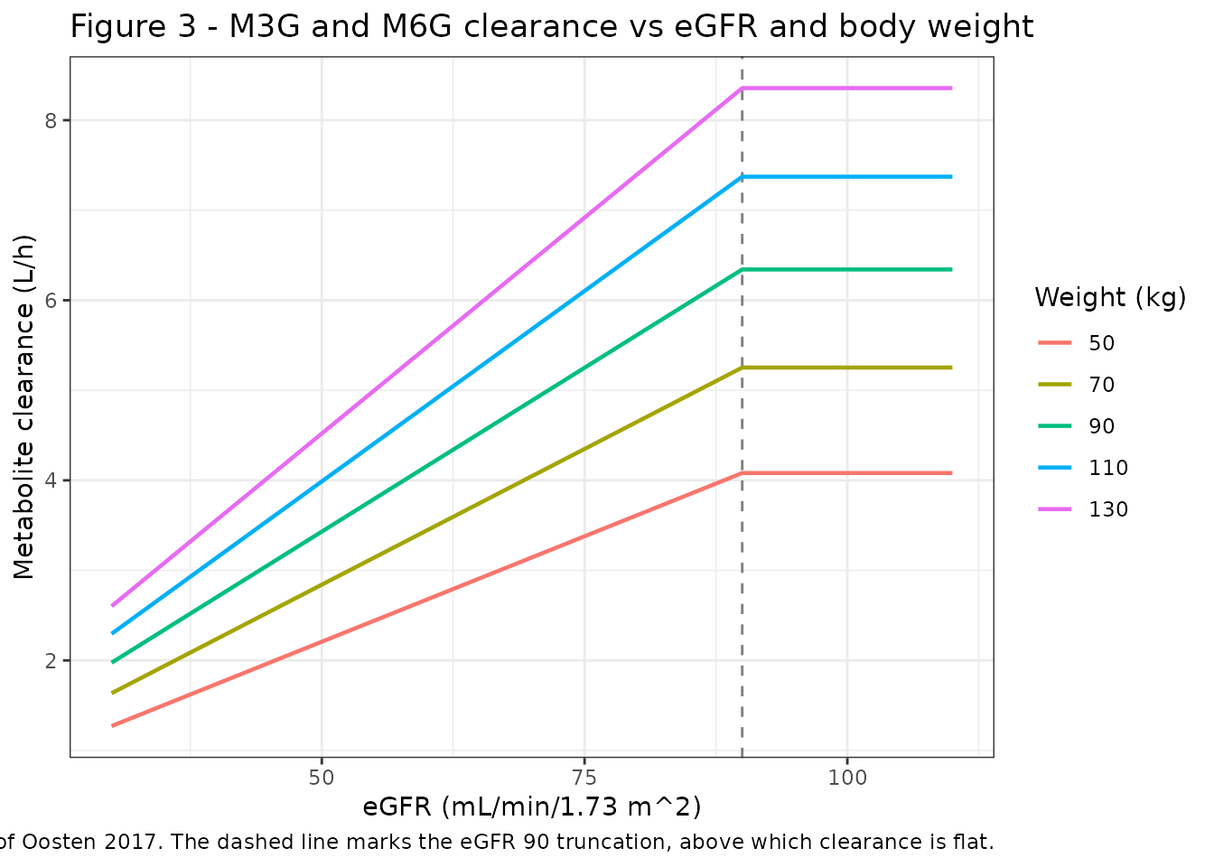

# Replicates Figure 4 of Oosten 2017: observed and simulated metabolite
# concentration ratios over time after dose, stratified by route. Oosten 2017
# pools both oral formulations into a single "Oral" panel.
ratios <- sim |>
  dplyr::filter(time > 0, Cc > 0, Cc_m6g > 0) |>
  dplyr::mutate(
    panel = ifelse(admin_arm == "Subcutaneous", "Subcutaneous", "Oral"),
    `M3G:M` = Cc_m3g / Cc,
    `M6G:M` = Cc_m6g / Cc,
    `M3G:M6G` = Cc_m3g / Cc_m6g
  ) |>
  tidyr::pivot_longer(c(`M3G:M`, `M6G:M`, `M3G:M6G`),
                      names_to = "ratio", values_to = "value") |>
  dplyr::mutate(ratio = factor(ratio, levels = c("M3G:M", "M6G:M", "M3G:M6G")))

ratios |>
  dplyr::group_by(panel, ratio, time) |>
  dplyr::summarise(
    Q05 = stats::quantile(value, 0.05),
    Q50 = stats::median(value),
    Q95 = stats::quantile(value, 0.95),
    .groups = "drop"
  ) |>
  ggplot(aes(time, Q50)) +
  geom_ribbon(aes(ymin = Q05, ymax = Q95), alpha = 0.25, fill = "firebrick") +
  geom_line(colour = "firebrick", linewidth = 0.7) +
  facet_grid(ratio ~ panel, scales = "free_y") +
  scale_x_log10() +
  scale_y_log10() +
  labs(
    x = "Time after dose (h)", y = "Concentration ratio",
    title = "Figure 4 - metabolite concentration ratios by route",
    caption = paste("Replicates Figure 4 of Oosten 2017. Line = simulated",
                    "median, band = 5th-95th percentile of the virtual cohort.")
  ) +
  theme_bw()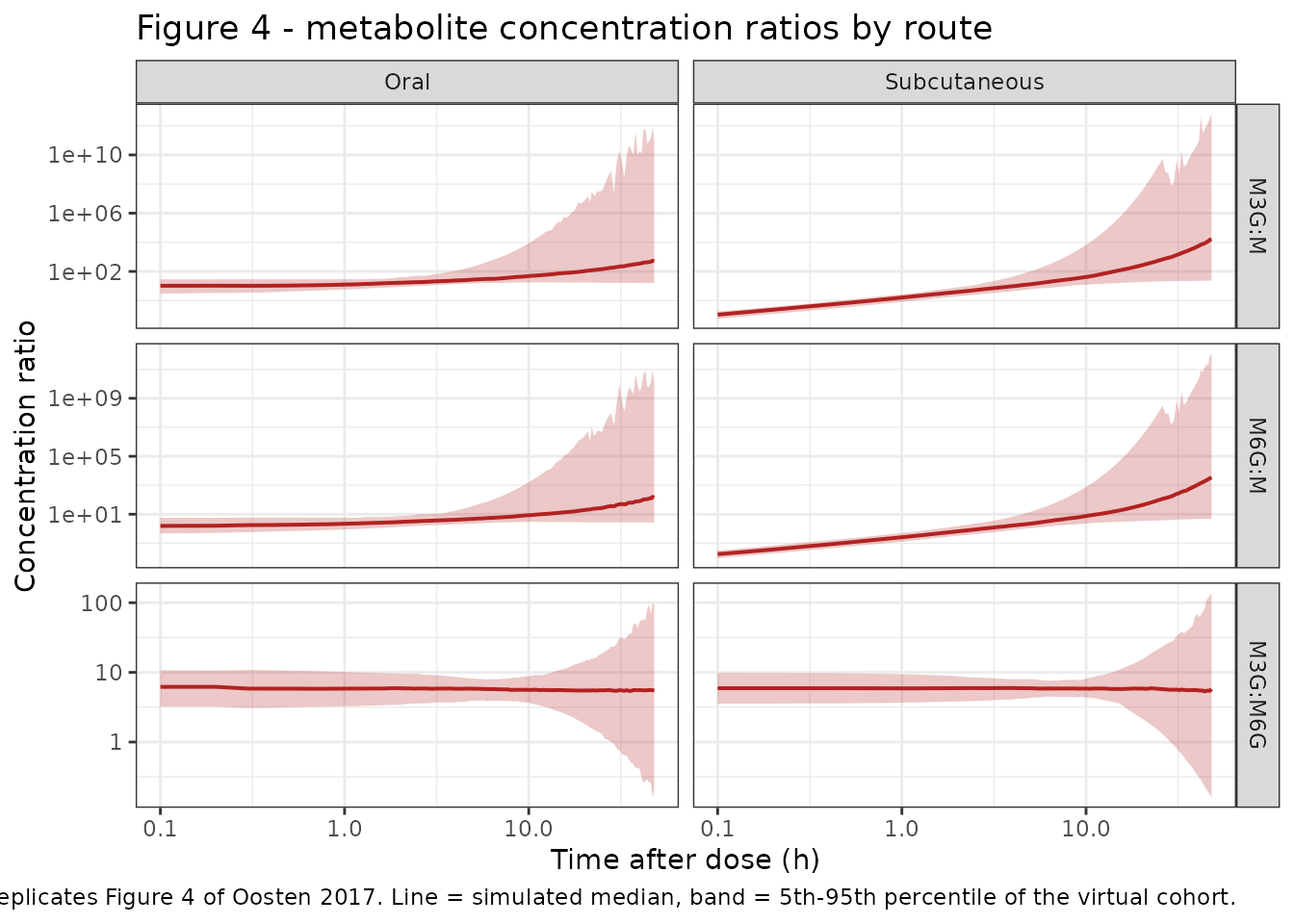

Oosten 2017 Figure 4 shows the two features this reproduces: the metabolite:morphine ratios are several-fold higher after oral than after subcutaneous morphine and rise with time after dose, whereas M3G:M6G is flat and nearly identical between routes. The M3G:M6G panels differ between the routes only by the first-pass contribution (5.70 subcutaneously against about 5.64 orally), which is why the paper describes it as “constant regardless of the level of renal impairment or route of administration”.

# Concentration-time profiles underlying the ratios above.
sim |>
  dplyr::filter(time > 0) |>
  tidyr::pivot_longer(c(Cc, Cc_m3g, Cc_m6g),
                      names_to = "analyte", values_to = "conc") |>
  dplyr::mutate(analyte = dplyr::recode(analyte, Cc = "Morphine",
                                        Cc_m3g = "M3G", Cc_m6g = "M6G")) |>
  dplyr::group_by(admin_arm, analyte, time) |>
  dplyr::summarise(
    Q05 = stats::quantile(conc, 0.05),
    Q50 = stats::median(conc),
    Q95 = stats::quantile(conc, 0.95),
    .groups = "drop"
  ) |>
  ggplot(aes(time, Q50, colour = analyte, fill = analyte)) +
  geom_ribbon(aes(ymin = Q05, ymax = Q95), alpha = 0.2, colour = NA) +
  geom_line(linewidth = 0.7) +
  facet_wrap(~admin_arm) +
  coord_cartesian(xlim = c(0, 48)) +
  labs(x = "Time after dose (h)", y = "Concentration (nmol/L)",
       colour = NULL, fill = NULL,
       title = "Simulated single-dose profiles by route") +
  theme_bw()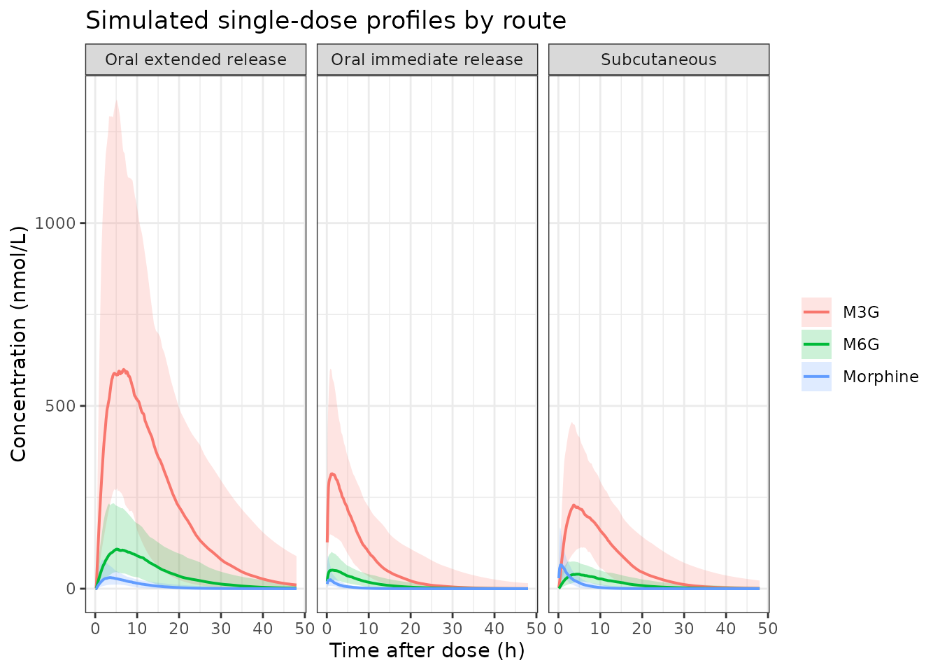

PKNCA validation

One PKNCA run per analyte, each grouped by route so per-route exposures can be compared. The dose object carries the morphine dose in nmol for every analyte; dose-normalised parameters are meaningful only for the morphine run.

dose_df <- events |>
  dplyr::filter(evid == 1L) |>
  dplyr::select(id, time, amt, admin_arm)

intervals <- data.frame(
  start = 0, end = Inf,
  cmax = TRUE, tmax = TRUE, auclast = TRUE, aucinf.obs = TRUE, half.life = TRUE
)

run_nca <- function(conc_col) {
  # Filter on !is.na() ONLY: adding `time > 0` or `conc > 0` would drop the
  # time-zero row PKNCA needs to anchor AUC0-*.
  d <- sim |>
    dplyr::filter(!is.na(.data[[conc_col]])) |>
    dplyr::transmute(id, time, admin_arm, Cc = .data[[conc_col]])
  d <- dplyr::bind_rows(
    d,
    d |> dplyr::distinct(id, admin_arm) |> dplyr::mutate(time = 0, Cc = 0)
  ) |>
    dplyr::distinct(id, admin_arm, time, .keep_all = TRUE) |>
    dplyr::arrange(id, admin_arm, time)

  conc_obj <- PKNCA::PKNCAconc(d, Cc ~ time | admin_arm + id)
  dose_obj <- PKNCA::PKNCAdose(dose_df, amt ~ time | admin_arm + id)
  PKNCA::pk.nca(PKNCA::PKNCAdata(conc_obj, dose_obj, intervals = intervals))
}

nca <- list(
  Morphine = run_nca("Cc"),
  M3G = run_nca("Cc_m3g"),
  M6G = run_nca("Cc_m6g")
)

nca_tbl <- dplyr::bind_rows(lapply(names(nca), function(a) {
  as.data.frame(nca[[a]]) |> dplyr::mutate(Analyte = a)
}))

nca_summary <- nca_tbl |>
  dplyr::filter(PPTESTCD %in% c("cmax", "tmax", "aucinf.obs", "half.life")) |>
  dplyr::group_by(Analyte, admin_arm, PPTESTCD) |>
  dplyr::summarise(Median = stats::median(PPORRES), .groups = "drop") |>
  tidyr::pivot_wider(names_from = PPTESTCD, values_from = Median)

nca_summary |>
  dplyr::relocate(Analyte, admin_arm, cmax, tmax, aucinf.obs, half.life) |>
  dplyr::rename(
    "Route" = admin_arm,
    "Cmax (nmol/L)" = cmax,
    "Tmax (h)" = tmax,
    "AUC0-inf (nmol*h/L)" = aucinf.obs,
    "t1/2 (h)" = half.life
  ) |>
  knitr::kable(digits = 2,
               caption = paste("Median non-compartmental parameters over the",
                               "virtual cohort, by analyte and route.",
                               "Oosten 2017 publishes no absolute NCA values;",
                               "the published comparison is the AUC-ratio",
                               "table above."))

Median non-compartmental parameters over the virtual cohort, by analyte and route. Oosten 2017 publishes no absolute NCA values; the published comparison is the AUC-ratio table above.
Analyte	Route	Cmax (nmol/L)	Tmax (h)	AUC0-inf (nmol*h/L)	t1/2 (h)
M3G	Oral extended release	642.75	6.0	11283.98	6.01
M3G	Oral immediate release	324.30	1.1	2943.74	4.44
M3G	Subcutaneous	237.65	4.6	3346.36	4.75
M6G	Oral extended release	110.23	6.1	1946.91	5.63
M6G	Oral immediate release	52.05	1.2	503.78	4.75
M6G	Subcutaneous	42.39	4.5	592.19	5.08
Morphine	Oral extended release	31.56	3.7	355.54	3.85
Morphine	Oral immediate release	25.44	0.5	NA	NA
Morphine	Subcutaneous	67.81	0.6	260.46	2.07

half_life <- function(analyte, rte) {
  nca_tbl |>
    dplyr::filter(Analyte == analyte, admin_arm == rte, PPTESTCD == "half.life") |>
    dplyr::pull(PPORRES) |>
    stats::median()
}

t_half_sc <- half_life("Morphine", "Subcutaneous")
t_half_met <- half_life("M3G", "Subcutaneous")

tibble::tibble(
  Claim = c(
    "Morphine terminal t1/2 within the 1.4-3.4 h literature range cited in the Introduction",
    "Metabolite t1/2 consistent with the model's ln(2) * Vmet / CLmet = 3.8 h"
  ),
  Achieved = c(t_half_sc, t_half_met)
) |>
  knitr::kable(digits = 2, caption = "Cohort-level half-life checks.")

Cohort-level half-life checks.
Claim	Achieved
Morphine terminal t1/2 within the 1.4-3.4 h literature range cited in the Introduction	2.07
Metabolite t1/2 consistent with the model’s ln(2) * Vmet / CLmet = 3.8 h	4.75


# Cohort medians, so these are robust-statistic bounds with headroom, not
# bounds read off one run. The subcutaneous arm is chosen because it has no
# flip-flop: ka,SC = 3.96 /h is far faster than kel = 91.9/278 = 0.33 /h.
stopifnot(
  t_half_sc > 1.4, t_half_sc < 3.4,
  t_half_met > 2.5, t_half_met < 6.0
)

# The extended-release arm is absorption-limited: ka,ER = 0.221 /h is SLOWER
# than morphine's elimination rate constant, so its apparent terminal half-life
# must exceed the subcutaneous one (flip-flop kinetics). This compares a large
# structural difference (ln2/0.221 = 3.1 h against 2.1 h), not two noisy
# statistics racing.
stopifnot(half_life("Morphine", "Oral extended release") > t_half_sc)

Cohort-level reproduction of the route contrast

per_subject <- sim |>
  dplyr::group_by(id, admin_arm) |>
  dplyr::summarise(
    a_m = PKNCA::pk.calc.auc.last(conc = Cc, time = time),
    a_3 = PKNCA::pk.calc.auc.last(conc = Cc_m3g, time = time),
    a_6 = PKNCA::pk.calc.auc.last(conc = Cc_m6g, time = time),
    .groups = "drop"
  ) |>
  dplyr::mutate(r_3m = a_3 / a_m, r_6m = a_6 / a_m, r_36 = a_3 / a_6)

cohort_tbl <- per_subject |>
  dplyr::group_by(admin_arm) |>
  dplyr::summarise(
    `M3G:morphine median` = stats::median(r_3m),
    `M6G:morphine median` = stats::median(r_6m),
    `M3G:M6G median` = stats::median(r_36),
    `M3G:M6G 5th-95th` = sprintf("%.2f - %.2f",
                                 stats::quantile(r_36, 0.05),
                                 stats::quantile(r_36, 0.95)),
    .groups = "drop"
  )
knitr::kable(cohort_tbl, digits = 2,
             caption = paste("Per-subject AUC ratios across the virtual",
                             "cohort. Typical-value ratios are in the table",
                             "further up; these carry between-subject",
                             "variability and so sit near, not on, them."))

Per-subject AUC ratios across the virtual cohort. Typical-value ratios are in the table further up; these carry between-subject variability and so sit near, not on, them.
admin_arm	M3G:morphine median	M6G:morphine median	M3G:M6G median	M3G:M6G 5th-95th
Oral extended release	30.40	5.46	5.74	4.17 - 7.59
Oral immediate release	29.87	5.06	5.76	4.35 - 7.48
Subcutaneous	12.27	2.04	5.91	4.61 - 7.18


sc_med <- cohort_tbl |> dplyr::filter(admin_arm == "Subcutaneous")
or_med <- cohort_tbl |> dplyr::filter(admin_arm == "Oral extended release")

# Centre-of-the-distribution assertions with generous headroom, chosen so they
# hold for ANY cohort this model can draw while still going red on a
# mis-transcribed fraction, clearance or dose (which move these medians by
# tens of per cent). M3G:M6G is the tightest because it is nearly free of
# between-subject variability: the two metabolites share CLmet and Vmet and
# their random effects are 0.912-correlated.
stopifnot(
  sc_med$`M3G:morphine median` > 7, sc_med$`M3G:morphine median` < 17,
  or_med$`M3G:morphine median` > 20, or_med$`M3G:morphine median` < 45,
  # The route contrast the paper highlights: oral first pass roughly triples
  # the M3G:morphine ratio.
  or_med$`M3G:morphine median` / sc_med$`M3G:morphine median` > 1.8,
  abs(sc_med$`M3G:M6G median` - 5.70) < 1.2,
  abs(or_med$`M3G:M6G median` - 5.65) < 1.2
)

Assumptions and deviations

Errata and value conflicts in the source

Fractions of morphine clearance forming each metabolite (fm_m3g, fm_m6g). The paper states two different pairs of values. Results 3.2 says “The fractions of total morphine clearance forming M3G and M6G were fixed to 0.57 and 0.10, respectively”, while Table 3 prints 0.573 fixed and 0.104 fixed. The model file uses 0.57 and 0.10, because the subcutaneous AUC ratios published in the same Results section have no first-pass term and so depend on nothing but these fractions and the CL/CLmet pair:

Published (Results 3.2)	With 0.57 / 0.10	With 0.573 / 0.104
M3G:morphine = 11.1	11.12	11.18
M6G:morphine = 1.95	1.95	2.03
M3G:M6G = 5.70	5.70	5.51

The M6G:morphine and M3G:M6G rows are far outside rounding, and the three oral ratios agree with the 0.57 / 0.10 reading as well (see the AUC-ratio table above, maximum deviation 0.21%). Two independent lines of evidence – the Results prose and all six of the paper’s own derived ratios – therefore point the same way, against Table 3’s two cells.

Morphine clearance. Table 3 gives CL 70kg = 91.9 L/h; the Discussion says “clearance in our study, estimated to be 92.9 L/h for a patient weighing 70 kg”. The model uses the tabulated 91.9, which is the value carrying the SIR confidence interval (85.8-99.9) and the value that reproduces the published AUC ratios (92.9 would put subcutaneous M6G:morphine at 1.97 rather than 1.95).

Structural interpretations

Where the first-pass metabolite enters. Figure 1 draws the first-pass arrows leaving the oral dose boxes without an absorption rate constant on them, so the diagram alone does not settle whether the first-pass metabolite appears as an instantaneous bolus in the metabolite compartment or is carried at the route’s own absorption rate. The model applies the four-way partition to the absorption flux out of each oral depot, i.e. at the route’s own ka (and, for the extended-release route, behind its lag time). Two reasons: every arrow in Figure 1, solid and dashed, leaves the dose box rather than bypassing it; and the odds-style parameterisation of Table 3 footnote b is the signature of competing first-order routes out of a shared compartment. The two readings give identical AUCs, AUC ratios and steady states – they differ only in the early metabolite profile after an extended-release dose, where a bolus reading would put metabolite in plasma before any parent had been absorbed.

Interindividual variability on absorption. Table 3 reports one IIV term for k a, all (71.0% CV) covering all three route-specific absorption rate constants, and the model applies a single etalka to all three accordingly. That row is reported with no SIR relative standard error and no confidence interval. Every other such NA row in Table 3 is either a fixed value or a derived quantity, and the subcutaneous and immediate-release absorption constants were themselves fixed from the literature, which suggests this variance was fixed too – but the paper never says so, so it is encoded here as estimated rather than fixed(). The distinction matters only to someone re-fitting the model.

eGFR truncation. The Methods truncate eGFR at 90 mL/min/1.73 m^2 in the dataset, and Results 3.2 states metabolite clearance is constant above that value. The model applies min(CRCL, 90) inside model() rather than relying on the input data being pre-truncated. Note that the covariate form is linear, not a power function, and goes negative below eGFR = 3.1 mL/min/1.73 m^2 – far below the observed 33 to >90 range, but the model must not be extrapolated there.

Not represented

Correlated residual errors. Oosten 2017 used the NONMEM L2 data item to estimate correlations between the three residual errors of one blood sample (morphine-M3G 0.420, morphine-M6G 0.386, M3G-M6G 0.918). nlmixr2 has no analogue, so those three off-diagonal $SIGMA terms are absent from the packaged model. They affect only the within-sample scatter of an observed concentration ratio; every concentration, AUC, AUC ratio and typical-value profile in this vignette is unaffected, because all three are computed from model predictions rather than from residual-perturbed observations.

Screened but unretained covariates. Age, sex, and the UGT2B7, SLC22A1 and ABCC3 polymorphisms were all tested and none reached p < 0.01 (Results 3.2 and 3.3). They are documented in the model file’s covariatesDataExcluded metadata rather than encoded. The one point estimate the paper prints for a rejected covariate – a 17.0% lower morphine clearance in women – carries no reported uncertainty and was not retained, so it is recorded in prose only.

Treatment failure. The paper tested treatment failure as a binary covariate on morphine and metabolite clearance and found no effect (Results 3.4); nothing is carried into the model.

Simulation assumptions

Covariate distributions are reconstructed from the Table 2 marginal summaries (median and range) because subject-level data are not public: weight log-normal about 83 kg clipped to 53-140 kg, eGFR normal about 81 clipped to 33-90. The paper reports no weight-eGFR correlation, and explicitly states that “no correlation was found between these two” for their effects on metabolite clearance, so they are drawn independently.
Single doses are simulated (10 mg subcutaneous, 40 mg oral extended release, 10 mg oral immediate release) so that “time after dose” on the Figure 4 replication means the same thing it does in the paper. The trial itself used continuous subcutaneous infusion and repeated oral dosing.
Doses are converted from the labelled salt weight to nmol of free base using the molecular weights the paper states (375.84 mg/mmol for morphine hydrochloride-3-water; 758.83 mg/mmol per two morphine for morphine 5-sulphate-water).
Every parameter value in the model file came from the paper’s own text, tables or figures. No value was taken from an external source, digitised from a plot, or obtained by correspondence.