Trastuzumab rezetecan (Gao 2026)

library(nlmixr2lib)
library(rxode2)
library(PKNCA)
library(dplyr)
library(ggplot2)

Gao X, Zhao K, Zhao Y, Zhang Y, Zhao J, Zhao C, Djebli N. Population Pharmacokinetics of Trastuzumab Rezetecan in Patients With HER2-Expressing or Mutated Advanced Solid Tumors. CPT Pharmacometrics Syst Pharmacol. 2026. doi:10.1002/psp4.70259. PMCID PMC13274680.

mod <- modellib("Gao_2026_trastuzumabRezetecan")
mod
#> function() {
#>   description <- "Sequential two-analyte population PK model for trastuzumab rezetecan (SHR-A1811, a HER2-targeting antibody-drug conjugate with a drug-to-antibody ratio of approximately 6.0; output Cc) and its released topoisomerase-I-inhibitor payload rezetecan (output Cc_rez) in adults with HER2-expressing or HER2-mutated advanced solid tumors (Gao 2026). The intact ADC is a two-compartment model with linear elimination after IV infusion. The released payload is a one-compartment model whose formation is a first-order release from the intact ADC in the central compartment and whose elimination is linear; the payload compartment does not feed back on the ADC, matching the paper's sequential two-step estimation. The release-rate constant Krel equals RAT during Cycle 1 and RAT * ALPHA (ALPHA = 0.693) from Cycle 2 onward. Covariates are body weight and baseline tumor size on ADC clearance; body weight, age and baseline albumin on ADC central volume; baseline albumin on ADC peripheral volume; body weight, baseline tumor size and cancer type on the release rate; age on payload volume; and aspartate aminotransferase on payload clearance."
#>   reference <- "Gao X, Zhao K, Zhao Y, Zhang Y, Zhao J, Zhao C, Djebli N. Population Pharmacokinetics of Trastuzumab Rezetecan in Patients With HER2-Expressing or Mutated Advanced Solid Tumors. CPT Pharmacometrics Syst Pharmacol. 2026. doi:10.1002/psp4.70259. PMCID PMC13274680."
#>   vignette <- "Gao_2026_trastuzumabRezetecan"
#> 
#>   # Gao 2026 reports intact-ADC concentrations in ug/mL (assay LLOQ 1.00
#>   # ug/mL) and released-payload concentrations in ng/mL (assay LLOQ 0.05
#>   # ng/mL). The ADC subsystem is encoded on the paper's own mass scale:
#>   # dose in mg and volumes in L give Cc directly in mg/L = ug/mL, which is
#>   # the scale the additive residual SD below is expressed on.
#>   #
#>   # The payload scale is NOT fully recoverable from the paper - see the
#>   # `mwr` note in model() and the vignette 'Assumptions and deviations'.
#>   units <- list(
#>     time = "day",
#>     dosing = "mg",
#>     concentration = "ug/mL"
#>   )
#> 
#>   # Issue #482: what each ODE state holds, in what amount units, in what
#>   # biological matrix.
#>   compartmentData <- list(
#>     central = list(analyte = "trastuzumab rezetecan (intact ADC)", units = "mg", specimen = "serum", verified = TRUE),
#>     peripheral1 = list(
#>       analyte = "trastuzumab rezetecan (intact ADC)",
#>       units = "mg",
#>       specimen = "serum",
#>       verified = TRUE
#>     ),
#>     central_rez = list(
#>       analyte = "released rezetecan payload",
#>       units = "mg ADC-molar-equivalent (see model() `mwr` note)",
#>       specimen = "serum",
#>       verified = TRUE
#>     )
#>   )
#> 
#>   covariateData <- list(
#>     WT = list(
#>       description = "Baseline body weight",
#>       units = "kg",
#>       type = "continuous",
#>       reference_category = NULL,
#>       notes = "Power effects on intact-ADC CL (exponent 0.525) and V1 (exponent 0.544), and on the payload release-rate constant RAT (exponent -0.546). Reference 60.6 kg, the value printed as the typical patient in the Gao 2026 Figure 5 and Figure 6 captions and appearing as the denominator of every body-weight term in the Section 3.2 and Section 3.3 equations. Dosing is weight-based (1.0-8.0 mg/kg), so ADC steady-state AUC scales as BW^(1 - 0.525) rather than BW^(-0.525).",
#>       source_name = "BW"
#>     ),
#>     AGE = list(
#>       description = "Baseline age",
#>       units = "years",
#>       type = "continuous",
#>       reference_category = NULL,
#>       notes = "Power effects on intact-ADC V1 (exponent 0.198) and on payload V3 (exponent 0.420). Reference 56 years (Gao 2026 Section 3.2 and 3.3 equations; the Figure 5 / Figure 6 captions define the typical patient as 56 years old).",
#>       source_name = "AGE"
#>     ),
#>     ALB = list(
#>       description = "Baseline serum albumin",
#>       units = "g/L",
#>       type = "continuous",
#>       reference_category = NULL,
#>       notes = "Power effects on intact-ADC V1 (exponent -0.363) and V2 (exponent -1.44); both volumes decrease as albumin rises. Reference 42.5 g/L (Gao 2026 Section 3.2 equations and the Figure 5 caption). Gao 2026 Table 1 abbreviation list confirms the unit is g/L, so no g/dL conversion is required.",
#>       source_name = "ALB"
#>     ),
#>     AST = list(
#>       description = "Baseline aspartate aminotransferase",
#>       units = "U/L",
#>       type = "continuous",
#>       reference_category = NULL,
#>       notes = "Power effect on released-payload clearance CL3 (exponent -0.167); payload clearance falls, and hence payload exposure rises, as AST rises. Reference 25 U/L (Gao 2026 Section 3.3 equation and the Figure 6 caption).",
#>       source_name = "AST"
#>     ),
#>     TUMSZ = list(
#>       description = "Baseline tumor size: sum of diameters of target lesions at baseline (RECIST)",
#>       units = "mm",
#>       type = "continuous",
#>       reference_category = NULL,
#>       notes = "Power effects on intact-ADC CL (exponent 0.0686) and on the payload release-rate constant RAT (exponent 0.100). Reference 52 mm (Gao 2026 Section 3.2 and 3.3 equations; the Figure 5 / Figure 6 captions give SOD 52 mm for the typical patient). Linear sum-of-diameters construct in mm, not an SPPD area. Source column SOD_B.",
#>       source_name = "SOD_B"
#>     ),
#>     TUMTP_BREAST = list(
#>       description = "Tumor-type indicator: 1 = breast cancer (BC), 0 = otherwise",
#>       units = "(binary)",
#>       type = "binary",
#>       reference_category = "0 (NSCLC is the model reference when TUMTP_BREAST, TUMTP_GASTRIC and TUMTP_OTHER are all 0)",
#>       notes = "Gao 2026 Table 1 note: 'CT1, CT2 and CT3 represent Breast Cancer (BC), Gastric or Gastroesophageal Junction cancer (GC/GEJ) and Other Tumor types, respectively.' The effect is ADDITIVE on the release-rate constant RAT (units 1/day), applied before the body-weight and tumor-size power terms: RAT_typical = 0.814 + 0.0562 for breast cancer. Breast cancer is the largest group in the analysis (approximately 60% of the 645 patients).",
#>       source_name = "CT1"
#>     ),
#>     TUMTP_GASTRIC = list(
#>       description = "Tumor-type indicator: 1 = gastric cancer or gastroesophageal junction (GEJ) adenocarcinoma, 0 = otherwise",
#>       units = "(binary)",
#>       type = "binary",
#>       reference_category = "0 (NSCLC is the model reference when TUMTP_BREAST, TUMTP_GASTRIC and TUMTP_OTHER are all 0)",
#>       notes = "Gao 2026 Table 1 CT2. ADDITIVE effect on the release-rate constant RAT (units 1/day): RAT_typical = 0.814 - 0.129 for GC/GEJ. The canonical TUMTP_GASTRIC register entry already covers gastric cancer OR adenocarcinoma of the gastroesophageal junction, which is exactly the Gao 2026 CT2 definition.",
#>       source_name = "CT2"
#>     ),
#>     TUMTP_OTHER = list(
#>       description = "Tumor-type indicator: 1 = other tumor types (neither NSCLC, breast, nor gastric/GEJ), 0 = otherwise",
#>       units = "(binary)",
#>       type = "binary",
#>       reference_category = "0 (NSCLC is the model reference when TUMTP_BREAST, TUMTP_GASTRIC and TUMTP_OTHER are all 0)",
#>       notes = "Gao 2026 Table 1 CT3. ADDITIVE effect on the release-rate constant RAT (units 1/day): RAT_typical = 0.814 + 0.0464 for other tumor types. NOTE the reference group here is NSCLC, NOT the 'other' pool: Gao 2026 Section 3.3 prints the NSCLC equation with the bare 0.814 and gives BC, GC/GEJ and Others their own additive shifts. This is the inverse orientation from papers that treat 'Other' as the residual reference, so the scope is paper-specific.",
#>       source_name = "CT3"
#>     ),
#>     CYCLE = list(
#>       description = "Treatment cycle number (1 = first 21-day cycle, 2 = second, ...; integer count, time-varying across the treatment course)",
#>       units = "(count)",
#>       type = "count",
#>       reference_category = "n/a -- used as the piecewise indicator CYCLE == 1 versus CYCLE >= 2",
#>       notes = "Required for the released-payload sub-model only. Gao 2026 Section 3.3: 'Krel = RAT during Cycle 1 and Krel = RAT * ALPHA after Cycle 1' with ALPHA = 0.693, i.e. the release rate drops to 69.3% of its Cycle-1 value from Cycle 2 onward. Cycle length is 21 days (Gao 2026 Section 2.1), so CYCLE increments every 21 days on the Q3W regimen. Does not affect intact-ADC disposition or payload elimination. Gao 2026 states that a release rate varying continuously with time or cycle was evaluated and did NOT improve the fit, so the step change is the paper's selected form.",
#>       source_name = "CYCLE"
#>     )
#>   )
#> 
#>   # Screened but not retained in the final model: Gao 2026 Section 3.4/3.5
#>   # and Figures S1-S7 report that race, sex, formulation, and hepatic and
#>   # renal function categories had no clinically relevant impact on either
#>   # analyte's exposure, so no point estimates are published for them.
#>   covariatesDataExcluded <- list(
#>     SEXF = list(
#>       description = "Sex (1 = female, 0 = male)",
#>       units = "(binary)",
#>       type = "binary",
#>       notes = "Assessed as a covariate and compared post hoc by subgroup (Gao 2026 Figure S4); not retained in the final model and no point estimate published."
#>     ),
#>     RACE_ASIAN = list(
#>       description = "Race indicator (1 = Asian, 0 = otherwise)",
#>       units = "(binary)",
#>       type = "binary",
#>       notes = "Ethnicity subgroups compared post hoc (Gao 2026 Figure S7); 'There is no remarkable difference in predicted exposures of Trastuzumab rezetecan between ethnicity groups'. Not retained; no point estimate published."
#>     ),
#>     CRCL = list(
#>       description = "Creatinine clearance (renal function category driver)",
#>       units = "mL/min",
#>       type = "continuous",
#>       notes = "Renal function categories compared post hoc (Gao 2026 Figure S1); no remarkable difference in exposure. Not retained; no point estimate published."
#>     ),
#>     HEPIMP_MILD = list(
#>       description = "Mild hepatic impairment indicator (NCI-ODWG)",
#>       units = "(binary)",
#>       type = "binary",
#>       notes = "Hepatic function categories compared post hoc (Gao 2026 Figure S2); no remarkable difference in exposure. Not retained; no point estimate published. AST was retained as a continuous covariate on payload clearance instead."
#>     )
#>   )
#> 
#>   population <- list(
#>     species = "human",
#>     n_subjects = 645,
#>     n_studies = 3,
#>     n_observations = "18,671 concentration records (9421 intact ADC, 9250 released payload) from 26,988 total records including 8317 dosing records",
#>     age_median = "56 years (typical-patient value used as the AGE covariate reference)",
#>     weight_median = "60.6 kg (typical-patient value used as the WT covariate reference); 5th percentile 45 kg, 95th percentile 82 kg",
#>     disease_state = "HER2-expressing or HER2-mutated advanced solid tumors: breast cancer (approximately 60% of the analysis population), gastric or gastroesophageal junction adenocarcinoma, colorectal cancer, and non-small cell lung cancer with HER2 expression, amplification or mutation.",
#>     dose_range = "1.0-8.0 mg/kg IV every 3 weeks (Q3W), 21-day treatment cycles.",
#>     studies = "Three phase 1 studies: SHR-A1811-I-101 (HER2-expressing or mutated advanced solid tumors), SHR-A1811-I-102 (HER2-expressing advanced gastric or gastroesophageal junction adenocarcinoma and colorectal cancer), and SHR-A1811-I-103 (advanced NSCLC with HER2 expression, amplification or mutation).",
#>     baseline_albumin_median = "42.5 g/L (typical-patient value used as the ALB covariate reference)",
#>     baseline_ast_median = "25 U/L (typical-patient value used as the AST covariate reference)",
#>     baseline_tumor_size_median = "52 mm sum of target-lesion diameters (typical-patient value used as the TUMSZ covariate reference); 5th percentile 15 mm, 95th percentile 149 mm",
#>     regions = "China (Jiangsu Hengrui Pharmaceuticals phase 1 programme)",
#>     notes = "Trastuzumab rezetecan (SHR-A1811) is a third-generation HER2-targeting ADC: anti-HER2 antibody trastuzumab, an enzyme-cleavable linker with a chiral cyclopropyl stabilising group, and the topoisomerase-I inhibitor payload rezetecan, at a drug-to-antibody ratio of approximately 6.0. Estimation used FOCE-I in NONMEM 7.5.1 with a SEQUENTIAL two-step approach: the intact-ADC fixed- and random-effect parameters were estimated first and then FIXED while the released-payload parameters were estimated. A one-step joint fit gave close estimates but ran about 6-fold longer. Gao 2026 Section 4 notes a trend toward nonlinear (TMDD-like) elimination at the 1.0 and 2.0 mg/kg dose levels (six patients each); a nonlinear component accounted for approximately 5% of total elimination and did not improve the fit, so linear clearance only was selected.",
#>     dosing_note = "Dose the `central` compartment only (IV infusion; Gao 2026 Figure 2). The released-payload compartment is driven by the intact-ADC central compartment and must NOT be dosed. Supply CYCLE as a time-varying covariate column that starts at 1 and increments every 21 days."
#>   )
#> 
#>   ini({
#>     # ============================================================
#>     # Intact ADC (trastuzumab rezetecan) -- Gao 2026 Table 1 and the
#>     # Section 3.2 equations. Two-compartment, linear elimination,
#>     # IV infusion (Gao 2026 Figure 2). No absorption parameter is
#>     # estimated; see the vignette Errata for the paper's stray
#>     # 'first-order absorption' wording in Section 3.2.
#>     # ============================================================
#>     lcl <- log(0.360); label("Intact ADC clearance (L/day)")                    # Gao 2026 Table 1: theta CL = 0.360 L/day (RSE 1.20%); Section 3.2 equation CL = 0.36 * ...
#>     lvc <- log(2.86);  label("Intact ADC central volume V1 (L)")                # Gao 2026 Table 1: theta V1 = 2.86 L (RSE 0.829%)
#>     lq  <- log(0.162); label("Intact ADC intercompartmental clearance Q (L/day)") # Gao 2026 Table 1: theta Q = 0.162 L/day (RSE 4.57%)
#>     lvp <- log(2.88);  label("Intact ADC peripheral volume V2 (L)")             # Gao 2026 Table 1: theta V2 = 2.88 L (RSE 4.34%)
#> 
#>     # Covariate effects on the intact ADC -- Gao 2026 Section 3.2 equations:
#>     #   CL = 0.36 * (BW/60.6)^0.525 * (SOD_B/52)^0.0686 * exp(eta_CL)
#>     #   V1 = 2.86 * (BW/60.6)^0.544 * (AGE/56)^0.198 * (ALB/42.5)^-0.363 * exp(eta_V1)
#>     #   Q  = 0.162 * exp(eta_Q)
#>     #   V2 = 2.88 * (ALB/42.5)^-1.44 * exp(eta_V2)
#>     e_wt_cl    <-  0.525;  label("Power exponent of WT on intact-ADC CL (unitless)")   # Gao 2026 Table 1: theta CL_BW = 0.525 (RSE 12.3%)
#>     e_tumsz_cl <-  0.0686; label("Power exponent of TUMSZ on intact-ADC CL (unitless)") # Gao 2026 Table 1: theta CL_SOD_B = 0.0686 (RSE 25.1%)
#>     e_wt_vc    <-  0.544;  label("Power exponent of WT on intact-ADC V1 (unitless)")   # Gao 2026 Table 1: theta V1_BW = 0.544 (RSE 8.05%)
#>     e_age_vc   <-  0.198;  label("Power exponent of AGE on intact-ADC V1 (unitless)")  # Gao 2026 Table 1: theta V1_AGE = 0.198 (RSE 17.9%)
#>     e_alb_vc   <- -0.363;  label("Power exponent of ALB on intact-ADC V1 (unitless)")  # Gao 2026 Table 1: theta V1_ALB = -0.363 (RSE 23.0%)
#>     e_alb_vp   <- -1.44;   label("Power exponent of ALB on intact-ADC V2 (unitless)")  # Gao 2026 Table 1: theta V2_ALB = -1.44 (RSE 31.6%)
#> 
#>     # ============================================================
#>     # Released payload (rezetecan) -- Gao 2026 Table 1 and the
#>     # Section 3.3 equations. One-compartment, first-order release
#>     # from the intact ADC, linear elimination.
#>     # ============================================================
#>     lkrel    <- log(0.814); label("Cycle-1 payload release-rate constant RAT from the intact ADC (1/day)") # Gao 2026 Table 1: theta RAT = 0.814 /day (RSE 3.12%)
#>     lfactor1 <- log(0.693); label("Multiplicative scaling ALPHA applied to the release rate from Cycle 2 onward (unitless)") # Gao 2026 Table 1: theta ALPHA = 0.693 (RSE 1.35%); Section 3.3 'Krel = RAT ( x ALPHA, if Cycle > 1)'
#>     lcl_rez  <- log(392);   label("Released-payload clearance CL3 (L/day)")     # Gao 2026 Table 1: theta CL3 = 392 L/day (RSE 2.46%)
#>     lvc_rez  <- fixed(log(30)); label("Released-payload volume of distribution V3 (L)")  # Gao 2026 Table 1: theta V3 = 30.0 Fix. Section 3.3: fixed 'similar to previously reported value of exatecan mesylate, to avoid identifiability issues'.
#> 
#>     # Covariate effects on the released payload -- Gao 2026 Section 3.3:
#>     #   NSCLC:    RAT = 0.814            * (BW/60.6)^-0.546 * (SOD_B/52)^0.1 * exp(eta_RAT)
#>     #   BC:       RAT = (0.814 + 0.0562) * (BW/60.6)^-0.546 * (SOD_B/52)^0.1 * exp(eta_RAT)
#>     #   GC/GEJ:   RAT = (0.814 - 0.129)  * (BW/60.6)^-0.546 * (SOD_B/52)^0.1 * exp(eta_RAT)
#>     #   Others:   RAT = (0.814 + 0.0464) * (BW/60.6)^-0.546 * (SOD_B/52)^0.1 * exp(eta_RAT)
#>     #   V3  = 30  * (AGE/56)^0.420  * exp(eta_V3)
#>     #   CL3 = 392 * (AST/25)^-0.167 * exp(eta_CL3)
#>     e_wt_krel    <- -0.546; label("Power exponent of WT on the payload release-rate constant (unitless)")    # Gao 2026 Table 1: theta RAT_BW = -0.546 (RSE 14.8%)
#>     e_tumsz_krel <-  0.100; label("Power exponent of TUMSZ on the payload release-rate constant (unitless)") # Gao 2026 Table 1: theta RAT_SOD_B = 0.100 (RSE 23.0%)
#> 
#>     # Cancer-type effects are ADDITIVE on the release-rate constant
#>     # (units 1/day) and are applied BEFORE the WT and TUMSZ power terms.
#>     # NSCLC is the reference (all three indicators zero).
#>     e_tumtp_breast_krel  <-  0.0562; label("Additive breast-cancer shift on the payload release-rate constant (1/day; vs NSCLC reference)")        # Gao 2026 Table 1: theta RAT_CT1 = 0.0562 /day (RSE 51.6%)
#>     e_tumtp_gastric_krel <- -0.129;  label("Additive gastric/GEJ-cancer shift on the payload release-rate constant (1/day; vs NSCLC reference)")   # Gao 2026 Table 1: theta RAT_CT2 = -0.129 /day (RSE 29.2%)
#>     e_tumtp_other_krel   <-  0.0464; label("Additive other-tumor-type shift on the payload release-rate constant (1/day; vs NSCLC reference)")     # Gao 2026 Table 1: theta RAT_CT3 = 0.0464 /day (RSE 78.0%)
#> 
#>     e_age_vc_rez <-  0.420; label("Power exponent of AGE on released-payload V3 (unitless)")  # Gao 2026 Table 1: theta V3_AGE = 0.420 (RSE 23.5%)
#>     e_ast_cl_rez <- -0.167; label("Power exponent of AST on released-payload CL3 (unitless)") # Gao 2026 Table 1: theta CL3_AST = -0.167 (RSE 26.9%)
#> 
#>     # ============================================================
#>     # Inter-individual variability. Gao 2026 Table 1 reports these as
#>     # omega^2 rows (variances on the log scale); the IIV was
#>     # 'described by an exponential model' (Section 2.3) and
#>     # 'assumed to have a lognormal distribution' (Section 3.2).
#>     # ============================================================
#>     etalcl ~ 0.0591                # Gao 2026 Table 1 row 'omega^2 CL' = 0.0591 (RSE 8.70%, shrinkage 8.60%)
#>     etalvc ~ 0.0408                # Gao 2026 Table 1 row 'omega^2 V1' = 0.0408 (RSE 23.5%, shrinkage 6.20%)
#>     etalq ~ 0.0798                 # Gao 2026 Table 1 row 'omega^2 Q' = 0.0798 (RSE 33.6%, shrinkage 56.0%)
#>     etalvp ~ 0.546                 # Gao 2026 Table 1 row 'omega^2 V2' = 0.546 (RSE 8.90%, shrinkage 21.6%)
#>     etalkrel ~ 0.0419              # Gao 2026 Table 1 row 'omega^2 RAT' = 0.0419 (RSE 25.3%, shrinkage 44.3%)
#>     etalfactor1 ~ 0.0692           # Gao 2026 Table 1 row 'omega^2 ALPHA' = 0.0692 (RSE 14.6%, shrinkage 20.0%)
#>     etalcl_rez ~ 0.140             # Gao 2026 Table 1 row 'omega^2 CL3' = 0.140 (RSE 14.5%, shrinkage 19.7%)
#>     etalvc_rez ~ 0.146             # Gao 2026 Table 1 row 'omega^2 V3' = 0.146 (RSE 13.3%, shrinkage 21.6%)
#> 
#>     # ============================================================
#>     # Residual variability. Gao 2026 Section 3.2: the intact-ADC
#>     # residual 'was best explained by a combined proportional and
#>     # additive error'; Table 1 note: 'residual variability (RUV),
#>     # included additive and proportional error terms for
#>     # Trastuzumab rezetecan and a proportional error term only for
#>     # released toxin.'
#>     #
#>     # The Table 1 RUV rows are NONMEM $SIGMA VARIANCES, on the same
#>     # 'Typical value' column as the omega^2 rows, so the SDs below
#>     # are square roots. Two independent checks support the variance
#>     # reading: (1) as SDs the proportional terms would be 3.13% and
#>     # 7.93% CV, implausibly tight for clinical bioanalytical assays
#>     # and irreconcilable with the spread in Gao 2026 Figure 1;
#>     # (2) as a variance the additive SD is sqrt(2.14) = 1.46 ug/mL,
#>     # about 1.5x the stated intact-ADC assay LLOQ of 1.00 ug/mL,
#>     # which is the expected magnitude.
#>     # ============================================================
#>     propSd     <- 0.176918; label("Intact-ADC proportional residual SD (fraction); sqrt(0.0313)")   # Gao 2026 Table 1 row 'Trastuzumab Rezetecan Prop RUV' = 0.0313 (variance; RSE 15.2%, shrinkage 6.90%)
#>     addSd      <- 1.462874; label("Intact-ADC additive residual SD (ug/mL); sqrt(2.14)")            # Gao 2026 Table 1 row 'Trastuzumab Rezetecan Add RUV' = 2.14 (variance; RSE 20.4%, shrinkage 6.90%)
#>     propSd_rez <- 0.281603; label("Released-payload proportional residual SD (fraction); sqrt(0.0793)") # Gao 2026 Table 1 row 'Toxin Rezetecan Prop RUV' = 0.0793 (variance; RSE 3.50%, shrinkage 8.50%)
#>   })
#>   model({
#>     # ============================================================
#>     # Individual parameters -- intact ADC (Gao 2026 Section 3.2)
#>     # ============================================================
#>     cl <- exp(lcl + etalcl) * (WT / 60.6)^e_wt_cl * (TUMSZ / 52)^e_tumsz_cl
#>     vc <- exp(lvc + etalvc) * (WT / 60.6)^e_wt_vc * (AGE / 56)^e_age_vc *
#>       (ALB / 42.5)^e_alb_vc
#>     q  <- exp(lq + etalq)
#>     vp <- exp(lvp + etalvp) * (ALB / 42.5)^e_alb_vp
#> 
#>     kel <- cl / vc
#>     k12 <- q / vc
#>     k21 <- q / vp
#> 
#>     # ============================================================
#>     # Individual parameters -- released payload (Gao 2026 Section 3.3)
#>     # ============================================================
#>     # Cancer-type shifts are additive on the release-rate constant and
#>     # precede the power terms, exactly as the four printed equations
#>     # show. NSCLC is the reference: with all three indicators zero the
#>     # typical release rate is the bare 0.814 /day.
#>     krel_typ <- exp(lkrel) +
#>       e_tumtp_breast_krel  * TUMTP_BREAST +
#>       e_tumtp_gastric_krel * TUMTP_GASTRIC +
#>       e_tumtp_other_krel   * TUMTP_OTHER
#> 
#>     # ALPHA applies from Cycle 2 onward; Cycle 1 uses the unscaled rate.
#>     factor1 <- exp(lfactor1 + etalfactor1)
#>     factor_krel <- factor1
#>     if (CYCLE < 2) factor_krel <- 1.0
#> 
#>     krel <- krel_typ * (WT / 60.6)^e_wt_krel * (TUMSZ / 52)^e_tumsz_krel *
#>       exp(etalkrel) * factor_krel
#> 
#>     cl_rez <- exp(lcl_rez + etalcl_rez) * (AST / 25)^e_ast_cl_rez
#>     vc_rez <- exp(lvc_rez + etalvc_rez) * (AGE / 56)^e_age_vc_rez
#> 
#>     kel_rez <- cl_rez / vc_rez
#> 
#>     # ------------------------------------------------------------
#>     # Molar-mass ratio for the payload formation term.
#>     #
#>     # Gao 2026 Section 3.3 states that 'the time course of intact
#>     # trastuzumab rezetecan concentrations, adjusted for the molar
#>     # mass, was the input to the released-payload model', but the
#>     # paper reports NO molecular weight for either the ADC or the
#>     # payload, and no drug-to-antibody-ratio multiplier appears in
#>     # the Figure 2 schematic or in any printed equation. `mwr` is
#>     # therefore held at 1, which makes `central_rez` an
#>     # ADC-molar-equivalent amount: the payload profile's SHAPE,
#>     # TIMING and every covariate RATIO are exact, while its absolute
#>     # mass concentration carries the unreported factor
#>     # MW_rezetecan / MW_ADC. Set `mwr` to that ratio to obtain mass
#>     # units. Nothing validated in the vignette depends on `mwr`,
#>     # because the payload residual error is purely proportional and
#>     # every published payload target is a ratio. This follows the
#>     # library precedent for an unreported payload scale constant in
#>     # `Lu_2022_patritumab.R` (V_DXd fixed to 1 L). See the vignette
#>     # 'Assumptions and deviations'.
#>     # ------------------------------------------------------------
#>     mwr <- 1.0
#> 
#>     # ============================================================
#>     # ODE system (Gao 2026 Figure 2). The ADC is dosed by IV
#>     # infusion into `central`. The Krel arrow into the payload
#>     # compartment is drawn DASHED in Figure 2 and the paper fitted
#>     # the two analytes sequentially with the ADC parameters fixed,
#>     # so payload formation does NOT deplete the ADC: the intact-ADC
#>     # disposition is exactly the two-compartment system above,
#>     # independent of Krel. This is the same forcing-function
#>     # structure used by Sathe_2024_sacituzumab.R.
#>     # ============================================================
#>     d/dt(central)     <- -kel * central - k12 * central + k21 * peripheral1
#>     d/dt(peripheral1) <-  k12 * central - k21 * peripheral1
#> 
#>     d/dt(central_rez) <-  krel * central * mwr - kel_rez * central_rez
#> 
#>     # ============================================================
#>     # Observations
#>     # ============================================================
#>     # Intact ADC: `central` in mg and `vc` in L give Cc in mg/L =
#>     # ug/mL, the unit Gao 2026 uses for the intact ADC throughout
#>     # (Figure 1A/C/E; assay LLOQ 1.00 ug/mL).
#>     Cc <- central / vc
#>     # Released payload in ADC-molar-equivalent ug/mL; multiply by
#>     # mwr = MW_rezetecan / MW_ADC and by 1000 to compare against the
#>     # ng/mL scale of Gao 2026 Figure 1B/D/F.
#>     Cc_rez <- central_rez / vc_rez
#> 
#>     Cc     ~ add(addSd) + prop(propSd)
#>     Cc_rez ~ prop(propSd_rez)
#>   })
#> }
#> <environment: 0x56151d823520>

Population

The analysis pooled 645 patients with HER2-expressing or HER2-mutated advanced solid tumors from three phase 1 studies (SHR-A1811-I-101, -I-102 and -I-103), contributing 18,671 concentration records (9421 intact ADC, 9250 released payload) out of 26,988 total records including 8317 dosing records (Gao 2026 Section 3.1). Trastuzumab rezetecan was given as an IV infusion every 3 weeks over a dose range of 1.0-8.0 mg/kg with a 21-day cycle length (Section 2.1). Breast cancer accounts for approximately 60% of the analysis population (Section 4).

The typical patient used as the covariate reference throughout the model is defined in the Gao 2026 Figure 5 and Figure 6 captions: a 56-year-old with body weight 60.6 kg, albumin 42.5 g/L, sum of target-lesion diameters 52 mm, and AST 25 U/L. Those same values appear as the denominators of every covariate term in the Section 3.2 and Section 3.3 equations.

Trastuzumab rezetecan (SHR-A1811) is a third-generation HER2-targeting antibody-drug conjugate: the anti-HER2 antibody trastuzumab, an enzyme-cleavable linker carrying a chiral cyclopropyl stabilising group, and the topoisomerase-I-inhibitor payload rezetecan, at a drug-to-antibody ratio of approximately 6.0.

Source trace

Every value in ini() and every equation in model() traces to the locations below. Gao 2026 Table 1 is the final-model parameter table with bootstrap medians and 95% CIs; the covariate equations are printed inline in Sections 3.2 (intact ADC) and 3.3 (released payload).

Quantity	Value	Source location
CL (L/day)	0.360	Table 1 theta CL; Section 3.2 equation
V1 (L)	2.86	Table 1 theta V1; Section 3.2 equation
Q (L/day)	0.162	Table 1 theta Q; Section 3.2 equation
V2 (L)	2.88	Table 1 theta V2; Section 3.2 equation
WT on CL	0.525	Table 1 theta CL_BW; (BW/60.6)^0.525
TUMSZ on CL	0.0686	Table 1 theta CL_SOD_B; (SOD_B/52)^0.0686
WT on V1	0.544	Table 1 theta V1_BW; (BW/60.6)^0.544
AGE on V1	0.198	Table 1 theta V1_AGE; (AGE/56)^0.198
ALB on V1	-0.363	Table 1 theta V1_ALB; (ALB/42.5)^-0.363
ALB on V2	-1.44	Table 1 theta V2_ALB; (ALB/42.5)^-1.44
RAT (1/day)	0.814	Table 1 theta RAT; Section 3.3 NSCLC equation
ALPHA	0.693	Table 1 theta ALPHA; Section 3.3 Krel = RAT (x ALPHA, if Cycle > 1)
CL3 (L/day)	392	Table 1 theta CL3; Section 3.3 equation
V3 (L), FIXED	30.0	Table 1 theta V3 ‘30.0 Fix’; Section 3.3 fixed to avoid identifiability issues
WT on RAT	-0.546	Table 1 theta RAT_BW; (BW/60.6)^-0.546
TUMSZ on RAT	0.100	Table 1 theta RAT_SOD_B; (SOD_B/52)^0.1
Breast cancer on RAT	+0.0562	Table 1 theta RAT_CT1; Section 3.3 BC equation (0.814 + 0.0562)
Gastric/GEJ on RAT	-0.129	Table 1 theta RAT_CT2; Section 3.3 GC/GEJ equation (0.814 - 0.129)
Other tumour on RAT	+0.0464	Table 1 theta RAT_CT3; Section 3.3 Others equation (0.814 + 0.0464)
AGE on V3	0.420	Table 1 theta V3_AGE; (AGE/56)^0.420
AST on CL3	-0.167	Table 1 theta CL3_AST; (AST/25)^-0.167
IIV variances	8 omega^2	Table 1 ‘Inter-individual variation’ block (omega^2 CL, V1, Q, V2, RAT, ALPHA, CL3, V3)
ADC residual	0.0313 / 2.14	Table 1 ‘Trastuzumab Rezetecan Prop RUV’ / ‘Add RUV’ (variances; see Assumptions)
Payload residual	0.0793	Table 1 ‘Toxin Rezetecan Prop RUV’ (variance; see Assumptions)
Model structure	2-cmt ADC + 1-cmt payload	Figure 2 schematic; Sections 3.2 and 3.3

Simulation setup

TAU     <- 21          # days per cycle (Gao 2026 Section 2.1)
N_CYC   <- 12          # cycles simulated; terminal t1/2 is ~20 days
DUR_INF <- 1.5 / 24    # assumed infusion duration, days (see Assumptions)
DOSE_MGKG <- 4.8       # the regimen Gao 2026 uses for all exposure comparisons

# Typical-patient covariate reference (Gao 2026 Figures 5 and 6 captions)
REF <- list(WT = 60.6, AGE = 56, ALB = 42.5, AST = 25, TUMSZ = 52)

LAST_START <- (N_CYC - 1) * TAU
LAST_END   <- N_CYC * TAU

# Typical-patient grid: dense enough around each infusion to resolve the
# end-of-infusion peak (Cmax) and the payload Tmax at 2-12 h, and dense
# enough over the final interval for a trapezoidal AUC that matches the
# closed-form Dose/CL to better than 0.1%.
TYP_TIMES <- sort(unique(c(
  seq(0, 2, by = 0.01),                          # first-dose peak + payload Tmax
  seq(0, 2 * TAU, by = 0.1),                     # cycles 1-2 step-down check
  seq(2 * TAU, LAST_START, by = 1),              # run-in to steady state
  seq(LAST_START, LAST_START + 2, by = 0.01),    # final-interval peak
  seq(LAST_START + 2, LAST_END, by = 0.1)
)))

# Cohort grid: lighter, since the cohort is used only for the VPC figure
# (first five cycles) and the final-interval NCA.
COHORT_TIMES <- sort(unique(c(
  seq(0, 5 * TAU, by = 0.5),
  seq(5 * TAU, LAST_START, by = 2),
  seq(LAST_START, LAST_START + 2, by = 0.05),
  seq(LAST_START + 2, LAST_END, by = 0.25)
)))

make_events <- function(WT = REF$WT, AGE = REF$AGE, ALB = REF$ALB,
                        AST = REF$AST, TUMSZ = REF$TUMSZ,
                        BREAST = 0, GASTRIC = 0, OTHER = 0,
                        mgkg = DOSE_MGKG, id = 1L, obs_times = TYP_TIMES) {
  doses <- rxode2::et(amt = mgkg * WT, dur = DUR_INF,
                      ii = TAU, addl = N_CYC - 1, cmt = "central")
  obs <- rxode2::et(obs_times)
  ev  <- as.data.frame(rbind(doses, obs))
  # The model declares two endpoints (Cc and Cc_rez), so observation records
  # must nominate one. Use dvid rather than cmt = "<observable>": naming an
  # observable as a compartment is what injects an extra cmt slot and
  # renumbers the ODE states. rxSolve still returns every model variable --
  # including Cc_rez and the individual cl -- as a column on these rows.
  ev$dvid  <- ifelse(is.na(ev$amt) | ev$amt == 0, 1L, NA_integer_)
  ev$id    <- id
  ev$WT    <- WT
  ev$AGE   <- AGE
  ev$ALB   <- ALB
  ev$AST   <- AST
  ev$TUMSZ <- TUMSZ
  ev$TUMTP_BREAST  <- BREAST
  ev$TUMTP_GASTRIC <- GASTRIC
  ev$TUMTP_OTHER   <- OTHER
  # Cycle 1 covers [0, 21); CYCLE increments every 21 days thereafter.
  ev$CYCLE <- pmax(1L, as.integer(floor(pmax(ev$time, 0) / TAU) + 1L))
  ev
}

trapz <- function(x, y) sum(diff(x) * (head(y, -1) + tail(y, -1)) / 2)

# AUC over the final (steady-state) dosing interval.
auc_ss <- function(sim, col) {
  w <- sim[sim$time >= LAST_START & sim$time <= LAST_END, ]
  trapz(w$time, w[[col]])
}

# Typical-value model: IIV suppressed, so every assertion below is
# deterministic and can be tight (an IIV cohort is handled separately).
typ <- rxode2::zeroRe(mod)
#> ℹ parameter labels from comments will be replaced by 'label()'

solve_typ <- function(...) {
  as.data.frame(rxode2::rxSolve(typ, make_events(...),
                                returnType = "data.frame"))
}

Structural checks on the typical patient

These run on zeroRe(mod), so they are deterministic: the two sides of each identity use the same parameters and differ only by solver error. They are the checks that catch a mis-transcribed clearance, volume, dose or unit.

Steady-state AUC equals Dose / CL

For a linear disposition model the AUC over a dosing interval at steady state is exactly Dose / CL, independent of the distribution parameters. This is the single strongest gate on CL and on the dose scaling.

typ_sim <- solve_typ()
#> ℹ omega/sigma items treated as zero: 'etalcl', 'etalvc', 'etalq', 'etalvp', 'etalkrel', 'etalfactor1', 'etalcl_rez', 'etalvc_rez'
auc_adc <- auc_ss(typ_sim, "Cc")
dose_mg <- DOSE_MGKG * REF$WT
cl_typ  <- 0.360      # Gao 2026 Table 1

closed_form <- tibble::tibble(
  `Simulated AUCss (ug*day/mL)` = auc_adc,
  `Dose / CL (ug*day/mL)`       = dose_mg / cl_typ,
  `Ratio`                       = auc_adc / (dose_mg / cl_typ)
)
knitr::kable(closed_form, digits = 4)

Simulated AUCss (ug*day/mL)	Dose / CL (ug*day/mL)	Ratio
807.9358	808	0.9999

# Pure numerical error: both sides use the same drawn parameters, so a tight
# bound is correct here (see the repo note on cohort-extreme assertions).
stopifnot(abs(auc_adc / (dose_mg / cl_typ) - 1) < 1e-3)

Intact-ADC concentrations match Gao 2026 Figure 1

Figure 1A/C/E plots mean intact-ADC concentrations by study and dose. At 4.8 mg/kg the observed profiles start at roughly 100-110 ug/mL, which is Dose / V1.

first_cycle <- typ_sim[typ_sim$time <= 1, ]
cmax_obs <- max(first_cycle$Cc)

fig1_tbl <- tibble::tibble(
  Quantity = c("Simulated Cmax, dose 1 (ug/mL)",
               "Dose / V1 (ug/mL)",
               "Gao 2026 Figure 1A at 4.8 mg/kg (ug/mL)"),
  Value    = c(sprintf("%.1f", cmax_obs),
               sprintf("%.1f", dose_mg / 2.86),
               "~100-110 (read from the figure)")
)
knitr::kable(fig1_tbl)

Quantity	Value
Simulated Cmax, dose 1 (ug/mL)	101.0
Dose / V1 (ug/mL)	101.7
Gao 2026 Figure 1A at 4.8 mg/kg (ug/mL)	~100-110 (read from the figure)

# Dose/V1 is an upper bound (elimination proceeds during the infusion).
stopifnot(cmax_obs > 90, cmax_obs <= dose_mg / 2.86)

Dose proportionality over 1.0-8.0 mg/kg

Gao 2026 Section 4: “The exposure (Cmax and AUC) of intact Trastuzumab Rezetecan increased proportionally over the dose range of 1.0-8.0 mg/kg.” The final model carries linear clearance only, so this must hold exactly.

dose_prop <- lapply(c(1.0, 2.0, 4.8, 8.0), function(d) {
  s <- solve_typ(mgkg = d)
  tibble::tibble(`Dose (mg/kg)` = d,
                 `AUCss (ug*day/mL)` = auc_ss(s, "Cc"),
                 `AUCss / dose` = auc_ss(s, "Cc") / (d * REF$WT))
}) |> bind_rows()
#> ℹ omega/sigma items treated as zero: 'etalcl', 'etalvc', 'etalq', 'etalvp', 'etalkrel', 'etalfactor1', 'etalcl_rez', 'etalvc_rez'
#> ℹ omega/sigma items treated as zero: 'etalcl', 'etalvc', 'etalq', 'etalvp', 'etalkrel', 'etalfactor1', 'etalcl_rez', 'etalvc_rez'
#> ℹ omega/sigma items treated as zero: 'etalcl', 'etalvc', 'etalq', 'etalvp', 'etalkrel', 'etalfactor1', 'etalcl_rez', 'etalvc_rez'
#> ℹ omega/sigma items treated as zero: 'etalcl', 'etalvc', 'etalq', 'etalvp', 'etalkrel', 'etalfactor1', 'etalcl_rez', 'etalvc_rez'
knitr::kable(dose_prop, digits = c(1, 1, 4))

Dose (mg/kg)	AUCss (ug*day/mL)	AUCss / dose
1.0	168.3	2.7776
2.0	336.6	2.7776
4.8	807.9	2.7776
8.0	1346.6	2.7776

stopifnot(diff(range(dose_prop$`AUCss / dose`)) / mean(dose_prop$`AUCss / dose`) < 1e-3)

Released-payload peak timing

Gao 2026 Section 4: the released payload shows “an initial increase and reaching peak concentrations within 2-12 h after dosing”.

tmax_rez_h <- 24 * first_cycle$time[which.max(first_cycle$Cc_rez)]
cat(sprintf("Simulated payload Tmax after dose 1: %.1f h (paper: 2-12 h)\n",
            tmax_rez_h))
#> Simulated payload Tmax after dose 1: 8.9 h (paper: 2-12 h)
stopifnot(tmax_rez_h >= 2, tmax_rez_h <= 12)

The Cycle-2 step down in release rate

Krel = RAT in Cycle 1 and RAT * ALPHA thereafter, with ALPHA = 0.693. The peak payload concentration does not fall by exactly the factor ALPHA because intact ADC accumulates between cycles, which partly offsets the lower release rate.

c1 <- typ_sim[typ_sim$time > 0 & typ_sim$time <= TAU, ]
c2 <- typ_sim[typ_sim$time > TAU & typ_sim$time <= 2 * TAU, ]
cycle_ratio <- max(c2$Cc_rez) / max(c1$Cc_rez)
cat(sprintf("Cycle-2 / Cycle-1 peak payload ratio: %.3f (ALPHA = 0.693)\n",
            cycle_ratio))
#> Cycle-2 / Cycle-1 peak payload ratio: 0.745 (ALPHA = 0.693)
# Must be a genuine step down, and bounded by ALPHA from below (accumulation
# can only raise the cycle-2 peak relative to a pure ALPHA scaling).
stopifnot(cycle_ratio < 1, cycle_ratio > 0.693)

Replicating the published covariate forest plots

Gao 2026 Figures 5 and 6 report the percentage change in steady-state exposure when each covariate is moved to its 5th or 95th percentile, with all other covariates held at the reference. Because dosing is weight-based, the body-weight effect on ADC AUC is the net of a proportional dose increase and a BW^0.525 clearance increase, i.e. BW^(1 - 0.525).

ref_auc_adc <- auc_ss(typ_sim, "Cc")

forest_adc <- bind_rows(
  lapply(list(list("Body weight 45 kg (5th pct)",  list(WT = 45),    -14.2),
              list("Body weight 82 kg (95th pct)", list(WT = 82),     16.8),
              list("Tumour size 15 mm (5th pct)",  list(TUMSZ = 15),  NA),
              list("Tumour size 149 mm (95th pct)", list(TUMSZ = 149), NA)),
         function(x) {
           s <- do.call(solve_typ, x[[2]])
           tibble::tibble(
             Scenario = x[[1]],
             `Simulated change in AUCss (%)` = 100 * (auc_ss(s, "Cc") / ref_auc_adc - 1),
             `Gao 2026 Figure 5 (%)` = x[[3]]
           )
         })
)
#> ℹ omega/sigma items treated as zero: 'etalcl', 'etalvc', 'etalq', 'etalvp', 'etalkrel', 'etalfactor1', 'etalcl_rez', 'etalvc_rez'
#> ℹ omega/sigma items treated as zero: 'etalcl', 'etalvc', 'etalq', 'etalvp', 'etalkrel', 'etalfactor1', 'etalcl_rez', 'etalvc_rez'
#> ℹ omega/sigma items treated as zero: 'etalcl', 'etalvc', 'etalq', 'etalvp', 'etalkrel', 'etalfactor1', 'etalcl_rez', 'etalvc_rez'
#> ℹ omega/sigma items treated as zero: 'etalcl', 'etalvc', 'etalq', 'etalvp', 'etalkrel', 'etalfactor1', 'etalcl_rez', 'etalvc_rez'
knitr::kable(forest_adc, digits = 2)

Scenario	Simulated change in AUCss (%)	Gao 2026 Figure 5 (%)
Body weight 45 kg (5th pct)	-13.19	-14.2
Body weight 82 kg (95th pct)	15.45	16.8
Tumour size 15 mm (5th pct)	8.90	NA
Tumour size 149 mm (95th pct)	-6.96	NA

The two body-weight scenarios reproduce the published direction and magnitude to within about 1.4 percentage points. The residual gap is expected: Gao 2026 generated the forest plot from 1000 simulated subjects drawn from the observed covariate distribution, whereas the rows above evaluate the model at a single covariate point. The tumour-size rows are both inside the paper’s stated envelope of “< 15%” (Section 3.4).

wt_rows <- forest_adc[!is.na(forest_adc$`Gao 2026 Figure 5 (%)`), ]
stopifnot(
  # Direction must match, and magnitude must land near the published value.
  all(sign(wt_rows$`Simulated change in AUCss (%)`) ==
        sign(wt_rows$`Gao 2026 Figure 5 (%)`)),
  max(abs(wt_rows$`Simulated change in AUCss (%)` -
            wt_rows$`Gao 2026 Figure 5 (%)`)) < 4
)
# Section 3.4: tumour size has "a slight impact on exposure < 15%".
tum_rows <- forest_adc[is.na(forest_adc$`Gao 2026 Figure 5 (%)`), ]
stopifnot(max(abs(tum_rows$`Simulated change in AUCss (%)`)) < 15)

For the released payload, Gao 2026 Section 4 states that elevated AST was associated with an 18.1% increase in payload AUCss at the 95th percentile. The paper does not print the AST 95th-percentile value, but the model’s payload AUC is proportional to (AST / 25)^0.167, so the published percentage identifies it. Recovering that value and feeding it back through the full ODE solve is a genuine round trip: it tests the payload formation term, the payload clearance covariate and the AUC integration together.

ref_auc_rez <- auc_ss(typ_sim, "Cc_rez")
ast_95 <- 25 * 1.181^(1 / 0.167)

payload_tbl <- bind_rows(
  lapply(
    list(
      list(sprintf("AST %.0f U/L (95th pct, recovered)", ast_95), list(AST = ast_95), 18.1),
      list("Breast cancer (vs NSCLC)",      list(BREAST = 1),  NA),
      list("Gastric / GEJ (vs NSCLC)",      list(GASTRIC = 1), NA),
      list("Other tumour type (vs NSCLC)",  list(OTHER = 1),   NA)
    ),
    function(x) {
      s <- do.call(solve_typ, x[[2]])
      tibble::tibble(
        Scenario = x[[1]],
        `Simulated change in payload AUCss (%)` =
          100 * (auc_ss(s, "Cc_rez") / ref_auc_rez - 1),
        `Gao 2026 (%)` = x[[3]]
      )
    })
)
#> ℹ omega/sigma items treated as zero: 'etalcl', 'etalvc', 'etalq', 'etalvp', 'etalkrel', 'etalfactor1', 'etalcl_rez', 'etalvc_rez'
#> ℹ omega/sigma items treated as zero: 'etalcl', 'etalvc', 'etalq', 'etalvp', 'etalkrel', 'etalfactor1', 'etalcl_rez', 'etalvc_rez'
#> ℹ omega/sigma items treated as zero: 'etalcl', 'etalvc', 'etalq', 'etalvp', 'etalkrel', 'etalfactor1', 'etalcl_rez', 'etalvc_rez'
#> ℹ omega/sigma items treated as zero: 'etalcl', 'etalvc', 'etalq', 'etalvp', 'etalkrel', 'etalfactor1', 'etalcl_rez', 'etalvc_rez'
knitr::kable(payload_tbl, digits = 2)

Scenario	Simulated change in payload AUCss (%)	Gao 2026 (%)
AST 68 U/L (95th pct, recovered)	18.10	18.1
Breast cancer (vs NSCLC)	6.90	NA
Gastric / GEJ (vs NSCLC)	-15.85	NA
Other tumour type (vs NSCLC)	5.70	NA

ast_row <- payload_tbl[!is.na(payload_tbl$`Gao 2026 (%)`), ]
stopifnot(abs(ast_row$`Simulated change in payload AUCss (%)` - 18.1) < 1)
# Section 4: "the resulting differences in payload exposure remained within 20%".
ct_rows <- payload_tbl[is.na(payload_tbl$`Gao 2026 (%)`), ]
stopifnot(max(abs(ct_rows$`Simulated change in payload AUCss (%)`)) < 20)

Typical-patient concentration-time profiles

typ_sim |>
  filter(time <= 5 * TAU) |>
  select(time, Cc, Cc_rez) |>
  tidyr::pivot_longer(c(Cc, Cc_rez), names_to = "analyte", values_to = "conc") |>
  mutate(analyte = recode(analyte,
                          Cc     = "Intact ADC (ug/mL)",
                          Cc_rez = "Released payload (ADC-molar-equivalent ug/mL)")) |>
  ggplot(aes(time, conc)) +
  geom_line(colour = "steelblue", linewidth = 0.8) +
  geom_vline(xintercept = TAU, linetype = "dashed", colour = "grey50") +
  facet_wrap(~ analyte, ncol = 1, scales = "free_y") +
  labs(x = "Time (day)", y = "Concentration",
       caption = "Dashed line marks the end of Cycle 1, where Krel steps down by ALPHA.")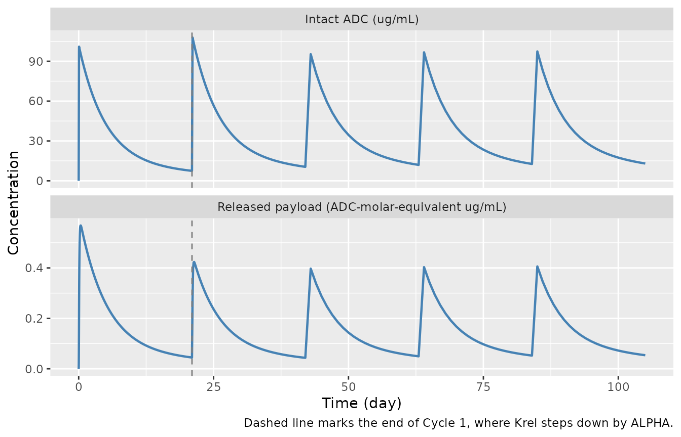

Typical-patient intact ADC (top) and released payload (bottom) profiles for trastuzumab rezetecan 4.8 mg/kg IV every 3 weeks. Qualitatively replicates Gao 2026 Figure 1A/B: the intact ADC declines biphasically and accumulates modestly across cycles, while the released payload tracks the ADC with a sharp early peak that steps down after Cycle 1 (Krel falls by the factor ALPHA = 0.693). The payload panel is in ADC-molar-equivalent units; see Assumptions and deviations.

Virtual cohort

A 200-subject cohort (the per-arm cap for this repository) with covariates drawn to match the reported reference values and percentiles. Body weight and tumour size are drawn log-normally and calibrated so their 5th and 95th percentiles land on the values Gao 2026 reports (45 and 82 kg; 15 and 149 mm).

rxode2::rxSetSeed(20260914)
set.seed(20260914)
N_SUBJ <- 200

# Log-normal calibrated to the reported 5th/95th percentiles.
lnorm_from_pctl <- function(n, p05, p95) {
  mu <- (log(p05) + log(p95)) / 2
  sd <- (log(p95) - log(p05)) / (2 * qnorm(0.95))
  rlnorm(n, mu, sd)
}

cohort <- tibble::tibble(
  id    = seq_len(N_SUBJ),
  WT    = lnorm_from_pctl(N_SUBJ, 45, 82),
  TUMSZ = lnorm_from_pctl(N_SUBJ, 15, 149),
  AGE   = pmin(pmax(rnorm(N_SUBJ, 56, 11), 20), 85),
  ALB   = pmin(pmax(rnorm(N_SUBJ, 42.5, 4.5), 25), 55),
  AST   = lnorm_from_pctl(N_SUBJ, 12, 67.7)
)
# Tumour-type mix: breast cancer is ~60% of the analysis population
# (Gao 2026 Section 4); the remainder is split across NSCLC (the model
# reference), gastric/GEJ and other tumour types.
ct <- sample(c("BREAST", "NSCLC", "GASTRIC", "OTHER"), N_SUBJ,
             replace = TRUE, prob = c(0.60, 0.15, 0.15, 0.10))
cohort$TUMTP_BREAST  <- as.integer(ct == "BREAST")
cohort$TUMTP_GASTRIC <- as.integer(ct == "GASTRIC")
cohort$TUMTP_OTHER   <- as.integer(ct == "OTHER")
cohort$cancer_type   <- ct

summary_tbl <- cohort |>
  summarise(
    `Body weight (kg)`     = sprintf("%.1f [%.0f, %.0f]", median(WT), quantile(WT, .05), quantile(WT, .95)),
    `Tumour size (mm)`     = sprintf("%.0f [%.0f, %.0f]", median(TUMSZ), quantile(TUMSZ, .05), quantile(TUMSZ, .95)),
    `Age (years)`          = sprintf("%.0f [%.0f, %.0f]", median(AGE), quantile(AGE, .05), quantile(AGE, .95)),
    `Albumin (g/L)`        = sprintf("%.1f [%.0f, %.0f]", median(ALB), quantile(ALB, .05), quantile(ALB, .95)),
    `AST (U/L)`            = sprintf("%.0f [%.0f, %.0f]", median(AST), quantile(AST, .05), quantile(AST, .95))
  ) |>
  tidyr::pivot_longer(everything(), names_to = "Covariate",
                      values_to = "Median [5th, 95th]")
knitr::kable(summary_tbl)

Covariate	Median [5th, 95th]
Body weight (kg)	61.1 [46, 86]
Tumour size (mm)	45 [16, 135]
Age (years)	57 [37, 76]
Albumin (g/L)	43.0 [35, 50]
AST (U/L)	30 [11, 75]

cohort_events <- bind_rows(lapply(seq_len(N_SUBJ), function(i) {
  r <- cohort[i, ]
  make_events(WT = r$WT, AGE = r$AGE, ALB = r$ALB, AST = r$AST,
              TUMSZ = r$TUMSZ, BREAST = r$TUMTP_BREAST,
              GASTRIC = r$TUMTP_GASTRIC, OTHER = r$TUMTP_OTHER,
              id = i, obs_times = COHORT_TIMES)
}))

cohort_sim <- as.data.frame(
  rxode2::rxSolve(mod, cohort_events, returnType = "data.frame")
)
#> ℹ parameter labels from comments will be replaced by 'label()'

cohort_sim |>
  filter(time <= 5 * TAU, !is.na(Cc)) |>
  group_by(time) |>
  summarise(med = median(Cc), lo = quantile(Cc, 0.05),
            hi = quantile(Cc, 0.95), .groups = "drop") |>
  ggplot(aes(time)) +
  geom_ribbon(aes(ymin = lo, ymax = hi), fill = "steelblue", alpha = 0.25) +
  geom_line(aes(y = med), colour = "steelblue", linewidth = 0.8) +
  scale_y_log10() +
  labs(x = "Time (day)", y = "Intact ADC (ug/mL)")
#> Warning in scale_y_log10(): log-10 transformation introduced infinite values.
#> log-10 transformation introduced infinite values.
#> log-10 transformation introduced infinite values.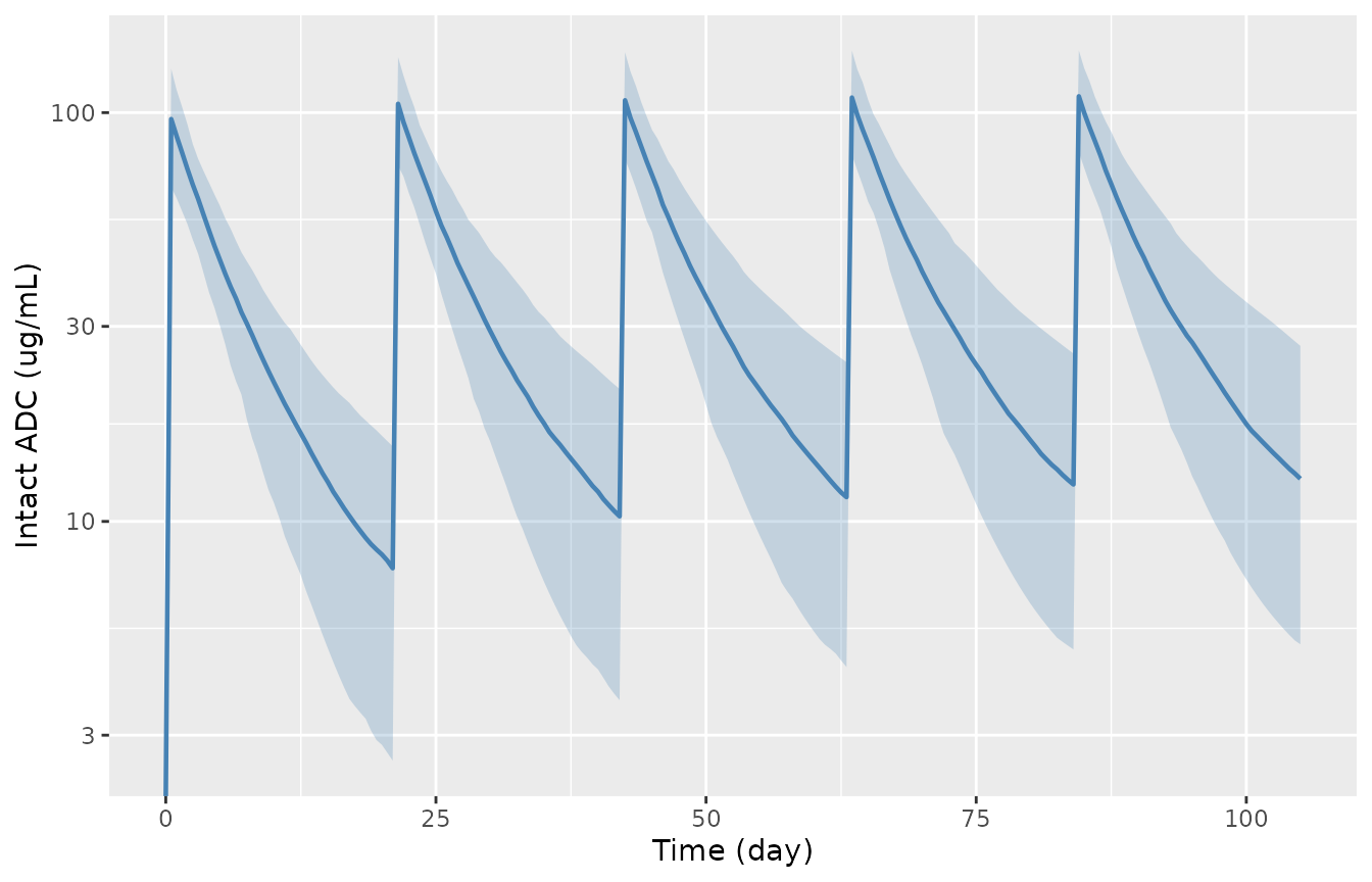

Simulated intact-ADC concentration-time profile over the first five cycles for the 200-subject virtual cohort: median (solid) with the 5th-95th percentile band. Compare with the prediction-corrected VPC in Gao 2026 Figure 4A.

PKNCA validation

Non-compartmental analysis of the final (steady-state) dosing interval for the intact ADC. The analysis is grouped by cancer type so per-group results can be compared, and the concentration frame is filtered only on !is.na(Cc) so the interval-start record is retained.

last_start <- LAST_START
last_end   <- LAST_END

conc_df <- cohort_sim |>
  filter(!is.na(Cc), time >= last_start, time <= last_end) |>
  left_join(select(cohort, id, cancer_type), by = "id") |>
  select(id, cancer_type, time, Cc)

# Defensive: guarantee a record exactly at the interval start and end.
stopifnot(
  all(tapply(conc_df$time, conc_df$id, min) == last_start),
  all(tapply(conc_df$time, conc_df$id, max) == last_end)
)

dose_df <- cohort |>
  transmute(id, cancer_type,
            time = last_start,
            dose = DOSE_MGKG * WT)

# Grouping variable first, then id, joined with `+` (PKNCAdose rejects a
# slash). Units are declared on both objects so the NCA output is not
# unit-blind.
o_conc <- PKNCA::PKNCAconc(conc_df, Cc ~ time | cancer_type + id,
                           concu = "ug/mL", timeu = "day")
o_dose <- PKNCA::PKNCAdose(dose_df, dose ~ time | cancer_type + id,
                           doseu = "mg")

intervals <- data.frame(
  start = last_start, end = last_end,
  cmax = TRUE, tmax = TRUE, auclast = TRUE, cmin = TRUE, half.life = TRUE
)

o_data <- PKNCA::PKNCAdata(o_conc, o_dose, intervals = intervals)
res <- suppressWarnings(PKNCA::pk.nca(o_data))
res_df <- as.data.frame(res)

nca_summary <- res_df |>
  filter(PPTESTCD %in% c("cmax", "tmax", "auclast", "cmin", "half.life")) |>
  group_by(PPTESTCD) |>
  summarise(Median = median(PPORRES, na.rm = TRUE),
            `5th`  = quantile(PPORRES, 0.05, na.rm = TRUE),
            `95th` = quantile(PPORRES, 0.95, na.rm = TRUE),
            .groups = "drop") |>
  rename("NCA parameter" = PPTESTCD)
knitr::kable(nca_summary, digits = 2)

NCA parameter	Median	5th	95th
auclast	828.64	522.27	1219.61
cmax	118.62	85.71	155.62
cmin	13.62	5.34	28.45
half.life	13.41	7.94	21.99
tmax	0.10	0.10	0.10

Gao 2026 does not publish a non-compartmental summary table for either analyte, so there is no side-by-side reference table to build. The NCA is instead used as an independent check on the model’s own arithmetic: for a linear model the steady-state interval AUC must equal Dose / CL_i subject-by-subject, where CL_i is the individual clearance rxode2 returns. This is a per-subject identity, not a cohort statistic, so it can be asserted tightly.

cl_i <- cohort_sim |>
  filter(!is.na(cl)) |>
  group_by(id) |>
  summarise(cl = first(cl), .groups = "drop")

mb <- res_df |>
  filter(PPTESTCD == "auclast") |>
  mutate(id = as.integer(as.character(id))) |>
  left_join(cl_i, by = "id") |>
  left_join(select(cohort, id, WT), by = "id") |>
  mutate(expected = DOSE_MGKG * WT / cl,
         pct_diff = 100 * (PPORRES / expected - 1))

mb_tbl <- tibble::tibble(
  `Median % difference`      = median(mb$pct_diff),
  `90th pctile |% diff|`     = quantile(abs(mb$pct_diff), 0.9),
  `Subjects`                 = nrow(mb)
)
knitr::kable(mb_tbl, digits = 3)

Median % difference	90th pctile |% diff|	Subjects
-0.071	2.821	200

stopifnot(
  nrow(mb) == N_SUBJ,
  !anyNA(mb$pct_diff),
  # Trapezoidal AUC on a 0.05-day grid slightly under-reads the post-infusion
  # peak, so the bias is small and negative rather than exactly zero.
  abs(median(mb$pct_diff)) < 2,
  quantile(abs(mb$pct_diff), 0.9) < 3
)

auc_by_ct <- res_df |>
  filter(PPTESTCD == "auclast") |>
  group_by(cancer_type) |>
  summarise(`Median AUCss (ug*day/mL)` = median(PPORRES, na.rm = TRUE),
            N = n(), .groups = "drop") |>
  rename("Cancer type" = cancer_type)
knitr::kable(auc_by_ct, digits = 1)

Cancer type	Median AUCss (ug*day/mL)	N
BREAST	825.3	131
GASTRIC	803.7	23
NSCLC	816.7	28
OTHER	855.6	18

Cancer type does not enter the intact-ADC model at all – it acts only on the payload release rate – so the intact-ADC AUC should not differ systematically across these groups beyond the body-weight and tumour-size imbalance that random sampling introduces.

The medians above still differ by roughly 20%, but that is covariate imbalance in small randomly drawn subgroups (N = 18 to 131), not a cancer-type effect. Asserting on those medians would be a cohort-extreme test that could pass here and fail on a CI runner with a different thread count. The structural claim – that cancer type does not enter the intact-ADC model at all – is instead tested deterministically on the typical-value model, where the four tumour-type settings must give bit-identical intact-ADC exposure while moving the payload exposure.

ct_settings <- list(NSCLC = list(), BREAST = list(BREAST = 1),
                    GASTRIC = list(GASTRIC = 1), OTHER = list(OTHER = 1))
ct_check <- bind_rows(lapply(names(ct_settings), function(nm) {
  s <- do.call(solve_typ, ct_settings[[nm]])
  tibble::tibble(`Cancer type` = nm,
                 `Intact ADC AUCss` = auc_ss(s, "Cc"),
                 `Payload AUCss`    = auc_ss(s, "Cc_rez"))
}))
#> ℹ omega/sigma items treated as zero: 'etalcl', 'etalvc', 'etalq', 'etalvp', 'etalkrel', 'etalfactor1', 'etalcl_rez', 'etalvc_rez'
#> ℹ omega/sigma items treated as zero: 'etalcl', 'etalvc', 'etalq', 'etalvp', 'etalkrel', 'etalfactor1', 'etalcl_rez', 'etalvc_rez'
#> ℹ omega/sigma items treated as zero: 'etalcl', 'etalvc', 'etalq', 'etalvp', 'etalkrel', 'etalfactor1', 'etalcl_rez', 'etalvc_rez'
#> ℹ omega/sigma items treated as zero: 'etalcl', 'etalvc', 'etalq', 'etalvp', 'etalkrel', 'etalfactor1', 'etalcl_rez', 'etalvc_rez'
knitr::kable(ct_check, digits = 4)

Cancer type	Intact ADC AUCss	Payload AUCss
NSCLC	807.9358	3.3252
BREAST	807.9354	3.5548
GASTRIC	807.9354	2.7983
OTHER	807.9354	3.5148

stopifnot(
  # Cancer type acts only on the payload release rate, so intact-ADC
  # exposure must be invariant across all four settings. The bound is not
  # exact zero because the payload state shares the ODE system, so changing
  # Krel perturbs the adaptive solver's step selection: the realised
  # relative spread is 4.3e-07, entirely solver tolerance. 1e-04 sits ~200x
  # above that noise and still ~500x below the smallest real covariate
  # effect in this model (the +5.7% "other tumour" payload shift), so a
  # genuine cancer-type leak into the ADC model would break it.
  diff(range(ct_check$`Intact ADC AUCss`)) /
    median(ct_check$`Intact ADC AUCss`) < 1e-4,
  # ... while payload exposure genuinely moves, confirming the indicators
  # are wired to the release rate rather than being silently ignored.
  diff(range(ct_check$`Payload AUCss`)) / median(ct_check$`Payload AUCss`) > 0.1
)

Assumptions and deviations

• Released-payload concentration scale is not fully recoverable. Gao 2026 Section 3.3 states that “the time course of intact trastuzumab rezetecan concentrations, adjusted for the molar mass, was the input to the released-payload model”, but the paper reports no molecular weight for either the ADC or the payload, and no drug-to-antibody-ratio multiplier appears in the Figure 2 schematic or in any printed equation. The model therefore holds the molar-mass ratio mwr at 1, which makes central_rez an ADC-molar-equivalent amount. The payload profile’s shape, timing and every covariate ratio are exact; only its absolute mass concentration carries the unreported factor MW_rezetecan / MW_ADC. Set mwr to that ratio to obtain mass units. Nothing asserted in this vignette depends on mwr, because the payload residual error is purely proportional and every published payload target is a ratio. A magnitude sanity check supports the one-to-one molar reading used here: with literature-scale molecular weights for an exatecan-class payload and a trastuzumab-based ADC, the simulated payload peak converts to roughly 2 ng/mL at 4.8 mg/kg, matching the approximately 2.5 ng/mL read from Gao 2026 Figure 1B, whereas a DAR-scaled (x6) formation term would predict about 12 ng/mL. This follows the library precedent for an unreported payload scale constant in Lu_2022_patritumab.R.
• Residual-error scale. Gao 2026 Table 1 lists the RUV rows in the same “Typical value” column as the omega^2 rows, and NONMEM $SIGMA is reported on the variance scale, so the model stores the square roots (propSd = sqrt(0.0313), addSd = sqrt(2.14), propSd_rez = sqrt(0.0793)). Two checks support this reading: read as SDs the proportional terms would be 3.13% and 7.93% CV, implausibly tight for clinical bioanalytical assays and irreconcilable with the spread in Figure 1; and read as a variance the additive SD is 1.46 ug/mL, about 1.5 times the stated intact-ADC assay LLOQ of 1.00 ug/mL, which is the expected magnitude.
• “First-order absorption” in Section 3.2 is a typographical error. Section 3.2 describes the intact ADC as “a two-compartment model with first-order absorption and elimination”, but Figure 2 shows the dose entering the central compartment by IV infusion, Table 1 contains no absorption-rate parameter, and no printed equation includes one. The model is encoded as IV, with no depot compartment.
• Infusion duration is assumed. The main text does not state the infusion duration (it is in Table S1, which is not available with the open-access deposit). The simulations use 1.5 h. This affects Cmax only; every AUC-based quantity, including all the forest-plot comparisons, is independent of it.
• Forest-plot percentages differ by about 1.4 percentage points. The body-weight rows reproduce Gao 2026 Figure 5 in direction and magnitude but not exactly (simulated -13.2% / +15.5% vs published -14.2% / +16.8%). The paper generated its forest plot from 1000 simulated subjects drawn from the observed covariate distribution, whereas this vignette evaluates the model at a single covariate point with all other covariates at their reference. No parameter was tuned to close the gap.
• The Section 3.3 payload equations print two different body-weight exponents. The NSCLC equation shows (BW/60.6)^-0.546 while the breast, gastric/GEJ and “other” equations show -0.545. Table 1 reports a single theta RAT_BW of -0.546, and the model has one such parameter, so -0.546 is used throughout; the -0.545 occurrences are a typesetting inconsistency. The difference is numerically immaterial (< 0.2% on the release rate).
• Cancer-type reference is NSCLC, not “other”. Gao 2026 prints the NSCLC release-rate equation with the bare 0.814 and gives breast, gastric/GEJ and “other” their own additive shifts. This is the inverse of the more common convention in which the “other” pool is the residual reference, and it is recorded in the TUMTP_OTHER register entry.
• Covariates screened but not retained. Race, sex, formulation, and hepatic and renal function categories were assessed and compared post hoc (Gao 2026 Figures S1-S7) but were not retained in the final model, and no point estimates are published for them. They are recorded in covariatesDataExcluded rather than covariateData.
• Nonlinear (TMDD) elimination is not implemented. Gao 2026 Section 4 notes a trend toward nonlinear elimination at 1.0 and 2.0 mg/kg (six patients each) but reports that a nonlinear component accounted for approximately 5% of total elimination and did not improve the fit, so the published final model carries linear clearance only. The model reproduces the paper’s selected structure.
• Sequential estimation is reflected in the structure. The paper fixed the intact-ADC parameters and then estimated only the payload parameters. Consistent with that and with the dashed Krel arrow in Figure 2, payload formation does not deplete the intact ADC, so intact-ADC disposition is exactly the two-compartment system regardless of Krel.
• The virtual cohort is constructed, not published. Gao 2026 reports the baseline covariate distributions in Tables S2 and S3, which are not available with the open-access deposit. The cohort here is drawn to match the reference values and the 5th/95th percentiles quoted in the main text (body weight 45/82 kg, tumour size 15/149 mm) and the approximately 60% breast-cancer share; it is not the paper’s actual covariate distribution.