Gentamicin in hypothermic HIE neonates (Sampson 2014)
Source:vignettes/articles/Sampson_2014_gentamicin.Rmd
Sampson_2014_gentamicin.RmdModel and source
- Citation: Sampson MR, Frymoyer A, Rattray B, Cotten CM, Smith B, Capparelli E, Bonifacio SL, Cohen-Wolkowiez M. Predictive performance of a gentamicin population pharmacokinetic model in neonates receiving full-body hypothermia. Ther Drug Monit. 2014;36(5):584-589.
- Article: https://doi.org/10.1097/FTD.0000000000000056
- Model origin: Frymoyer A, Lee S, Bonifacio SL, Meng L, Lucas SS, Guglielmo BJ, Sun Y, Verotta D. Every 36-h gentamicin dosing in neonates with hypoxic-ischemic encephalopathy receiving hypothermia. J Perinatol. 2013;33(10):778-782. https://doi.org/10.1038/jp.2013.59
mod_meta <- rxode2::rxode(readModelDb("Sampson_2014_gentamicin"))
#> ℹ parameter labels from comments will be replaced by 'label()'
mod_meta$description
#> [1] "One-compartment IV population PK model of gentamicin in term neonates with hypoxic-ischaemic encephalopathy undergoing whole-body hypothermia, as reported (model originally developed by Frymoyer 2013; this model file reproduces the parameter values stated by Sampson 2014 during the model's external predictive-performance evaluation). Allometric body-weight scaling on CL (fixed exponent 0.75) and linear body-weight scaling on V (exponent 1) referenced to a 3.3 kg neonate, with a power effect of serum creatinine on CL (exponent -0.566); inter-individual variability on CL only and proportional residual error."
mod_meta$reference
#> [1] "Sampson MR, Frymoyer A, Rattray B, Cotten CM, Smith B, Capparelli E, Bonifacio SL, Cohen-Wolkowiez M. Predictive performance of a gentamicin population pharmacokinetic model in neonates receiving full-body hypothermia. Ther Drug Monit. 2014;36(5):584-589. doi:10.1097/FTD.0000000000000056. Model originally developed in Frymoyer A, Lee S, Bonifacio SL, Meng L, Lucas SS, Guglielmo BJ, Sun Y, Verotta D. Every 36-h gentamicin dosing in neonates with hypoxic-ischemic encephalopathy receiving hypothermia. J Perinatol. 2013;33(10):778-782. doi:10.1038/jp.2013.59 (PMID 23553582); the present file reproduces the parameter values stated in Sampson 2014 Methods (page 585)."
mod_meta$units
#> $time
#> [1] "hour"
#>
#> $dosing
#> [1] "mg"
#>
#> $concentration
#> [1] "mg/L"
Population
The packaged model reproduces the one-compartment IV gentamicin popPK model originally developed by Frymoyer 2013 in 29 term neonates with hypoxic-ischaemic encephalopathy (HIE) undergoing whole-body hypothermia at UCSF (median gestational age 40 weeks, range 36-42; median postnatal age 2 days, range 1-4; 47 plasma gentamicin concentrations). Sampson 2014 then evaluated the predictive performance of that model on two external retrospective cohorts that used the same standard NICHD hypothermia protocol (33.5 degC for 72 h initiated within 6 h of birth, followed by 8 h of rewarming):
- Validation A – 18 UCSF neonates (33 samples) treated 2011-2012, dosed 5 mg/kg q36h. Median GA 40 weeks (38-42), median birth weight 3.4 kg (1.9-4.0), median SCR 1.0 mg/dL (0.6-1.3) at the first sample.
- Validation B – 23 Duke neonates (43 samples, 76% within 96 h of birth) treated 2006-2008, dosed 3.5-4 mg/kg q24h or q36h. Median GA 39 weeks (33-41), median birth weight 3.5 kg (2.5-4.6), median SCR 1.0 mg/dL (0.4-1.9) at the first sample.
According to Sampson 2014, the model adequately predicted Validation A concentrations (median AFE 1.1, NPDE p > 0.05, 88% of observations inside the 90% prediction interval) but systematically under-predicted Validation B (median AFE 0.6, NPDE p < 0.05, 50% inside the 90% prediction interval). Differences in serum-creatinine assay (Jaffe vs enzymatic) and dataset structure (initial peak + trough only vs multiple post-therapy samples) were hypothesised as drivers of the inter-institutional gap.
The same metadata is available programmatically via
readModelDb("Sampson_2014_gentamicin")$population.
Source trace
The per-parameter origin is recorded as an in-file comment next to
each ini() entry in
inst/modeldb/specificDrugs/Sampson_2014_gentamicin.R. The
table below collects them in one place for review.
| Equation / parameter | Value | Source location |
|---|---|---|
lcl (log CL at BW=3.3 kg, SCR=1 mg/dL) |
log(0.111) | Sampson 2014 page 585 (Frymoyer 2013 final model) |
lvc (log V at BW=3.3 kg) |
log(1.56) | Sampson 2014 page 585 (Frymoyer 2013 final model) |
e_wt_cl (allometric exponent on CL) |
0.75 (fixed) | Sampson 2014 page 585: (BW/3.3)^0.75 (theoretical
allometry) |
e_wt_vc (linear exponent on V) |
1 (fixed) | Sampson 2014 page 585: V = 1.56 * (BW/3.3)
|
e_creat_cl (power exponent of (1/CREAT) on
CL) |
0.566 | Sampson 2014 page 585: (1/SCR(mg/dL))^0.566
|
| IIV CL (omega^2 = log(1 + 0.161^2)) | 0.025591 (16.1% CV) | Sampson 2014 page 585: “estimate of inter-individual variability in CL was 16.1%” |
propSd (proportional residual SD) |
0.162 | Sampson 2014 page 585: “residual variability (proportional error model) was 16.2%” |
| One-compartment IV PK ODE structure | n/a | Sampson 2014 page 585: “Gentamicin PK was characterized with a one-compartment model” |
| Reference body weight 3.3 kg | n/a | Sampson 2014 page 585: (BW/3.3) normalisation; cohort
median BW 3.3 kg (Table 1) |
| Implicit reference SCR 1 mg/dL | n/a | Sampson 2014 page 585: (1/SCR(mg/dL))^0.566 – SCR is
absorbed without a reference divisor, so the factor equals 1 when SCR =
1 mg/dL |
Virtual cohort
Original observed data from the Frymoyer 2013 development cohort and the Sampson 2014 validation cohorts are not publicly available. The vignette draws three virtual cohorts that span the two institutional dosing regimens evaluated in Sampson 2014, and a typical-WT pediatric HIE patient:
- “UCSF 5 mg/kg q36h” – Validation A regimen (BW 3.4 kg, SCR 1.0 mg/dL).
- “Duke 4 mg/kg q24h” – Validation B regimen (BW 3.5 kg, SCR 1.0 mg/dL).
- “Duke 4 mg/kg q36h” – Validation B alternate regimen (BW 3.5 kg, SCR 1.0 mg/dL).
Body weight and serum creatinine are held constant at each cohort’s reported median to keep the simulated typical profile visible; users wanting full IIV / IOV / covariate variation can extend the cohort builder.
set.seed(20260621)

n_subjects <- 100L
infusion_h <- 0.5      # 30 min infusion per standard NICU gentamicin protocol
duration_h <- 4 * 24   # 4-day window covers >= 2 doses of each regimen

regimens <- tibble::tribble(
  ~regimen,               ~wt_kg, ~creat_mg_per_dl, ~dose_mg_per_kg, ~interval_h,
  "UCSF 5 mg/kg q36h",    3.4,    1.0,              5,               36,
  "Duke 4 mg/kg q24h",    3.5,    1.0,              4,               24,
  "Duke 4 mg/kg q36h",    3.5,    1.0,              4,               36
)

obs_grid <- sort(unique(c(
  seq(0, 2, by = 0.1),                # peri-peak resolution
  seq(2, duration_h, by = 1)          # hourly through 4 days
)))

make_cohort <- function(n, regimen, wt_kg, creat_mg_per_dl,
                        dose_mg_per_kg, interval_h, id_offset = 0L) {
  ids        <- id_offset + seq_len(n)
  amt_mg     <- wt_kg * dose_mg_per_kg
  dose_times <- seq(0, duration_h - 1, by = interval_h)

  dose_rows <- tidyr::expand_grid(id = ids, time = dose_times) |>
    dplyr::mutate(
      evid    = 1L,
      cmt     = "central",
      amt     = amt_mg,
      rate    = amt_mg / infusion_h,
      WT      = wt_kg,
      CREAT   = creat_mg_per_dl,
      regimen = regimen
    )

  obs_rows <- tidyr::expand_grid(id = ids, time = obs_grid) |>
    dplyr::mutate(
      evid    = 0L,
      cmt     = "central",
      amt     = 0,
      rate    = 0,
      WT      = wt_kg,
      CREAT   = creat_mg_per_dl,
      regimen = regimen
    )

  dplyr::bind_rows(dose_rows, obs_rows) |>
    dplyr::arrange(id, time, dplyr::desc(evid))
}

events <- dplyr::bind_rows(
  Map(function(i) make_cohort(
        n_subjects,
        regimens$regimen[i],
        regimens$wt_kg[i],
        regimens$creat_mg_per_dl[i],
        regimens$dose_mg_per_kg[i],
        regimens$interval_h[i],
        id_offset = (i - 1L) * 1000L
      ),
      seq_len(nrow(regimens)))
)

stopifnot(!anyDuplicated(unique(events[, c("id", "time", "evid")])))

cat(
  "Dose rows:", sum(events$evid == 1L),
  " | Obs rows:", sum(events$evid == 0L),
  " | Subjects:", n_subjects * nrow(regimens), "\n"
)
#> Dose rows: 1000  | Obs rows: 34500  | Subjects: 300
Simulation
mod <- readModelDb("Sampson_2014_gentamicin")
sim <- rxode2::rxSolve(
  mod,
  events = events,
  keep   = c("regimen", "WT", "CREAT")
) |>
  as.data.frame()
#> ℹ parameter labels from comments will be replaced by 'label()'
Concentration-time profiles
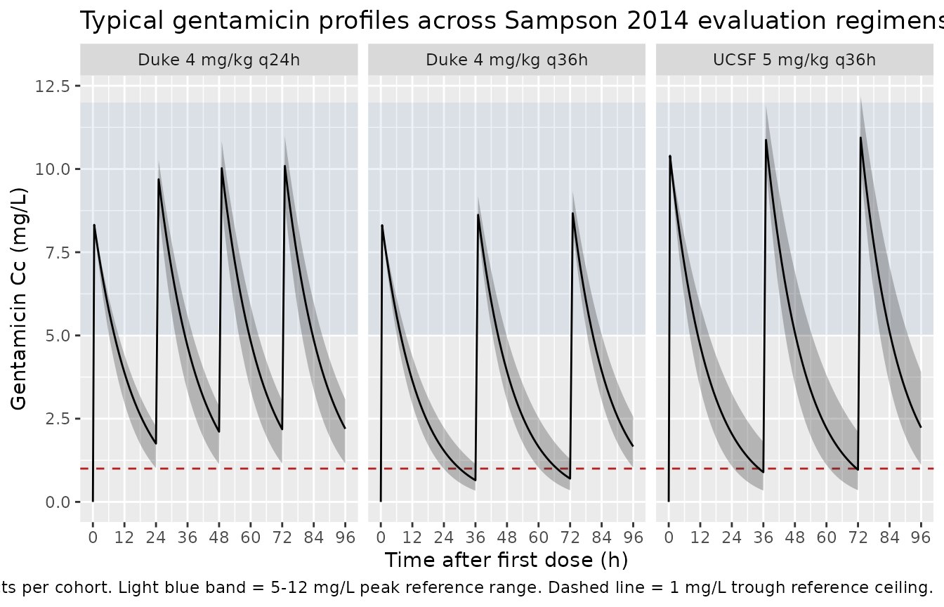
Sampson 2014 reports VPCs of observed vs. simulated concentrations in its Figure 2 across Validation A and Validation B. The figure cannot be faithfully reproduced without the underlying observed data, but the chunk below shows the analogous typical-value plus 5th-95th percentile envelope for the three regimens evaluated in the paper. The envelope illustrates the expected gentamicin exposure given the model and a typical neonate at each regimen’s reported median demographics.
ribbon_df <- sim |>
  dplyr::filter(!is.na(Cc)) |>
  dplyr::group_by(regimen, time) |>
  dplyr::summarise(
    Q05 = quantile(Cc, 0.05, na.rm = TRUE),
    Q50 = quantile(Cc, 0.50, na.rm = TRUE),
    Q95 = quantile(Cc, 0.95, na.rm = TRUE),
    .groups = "drop"
  )

ggplot(ribbon_df, aes(time, Q50)) +
  annotate("rect", xmin = -Inf, xmax = Inf, ymin = 5, ymax = 12,
           alpha = 0.10, fill = "steelblue") +
  geom_hline(yintercept = 1, linetype = "dashed", colour = "firebrick") +
  geom_ribbon(aes(ymin = Q05, ymax = Q95), alpha = 0.30) +
  geom_line() +
  facet_wrap(~regimen, ncol = 3) +
  scale_x_continuous(breaks = seq(0, 96, 12)) +
  labs(
    x       = "Time after first dose (h)",
    y       = "Gentamicin Cc (mg/L)",
    title   = "Typical gentamicin profiles across Sampson 2014 evaluation regimens",
    caption = paste0(
      "Median (solid) and 5th-95th percentile (shaded) gentamicin profiles ",
      "across ", n_subjects, " virtual subjects per cohort. ",
      "Light blue band = 5-12 mg/L peak reference range. ",
      "Dashed line = 1 mg/L trough reference ceiling."
    )
  )
PKNCA validation
Compute Cmax (peak) and Cmin (trough) per subject over the final
dosing interval in the simulation using PKNCA, grouped by
regimen. Peak occurs at the end of the 30-min infusion
(t = 0.5 h after dose start); trough occurs immediately
before the next dose.
last_dose_start <- vapply(regimens$interval_h, function(int) {
  starts <- seq(0, duration_h - 1, by = int)
  max(starts[starts + int <= duration_h])
}, numeric(1))
names(last_dose_start) <- regimens$regimen
last_dose_end <- last_dose_start + regimens$interval_h
names(last_dose_end) <- regimens$regimen

sim_nca <- sim |>
  dplyr::filter(!is.na(Cc)) |>
  dplyr::group_by(regimen) |>
  dplyr::mutate(
    interval_start = last_dose_start[as.character(regimen)],
    interval_end   = last_dose_end[as.character(regimen)]
  ) |>
  dplyr::filter(time >= interval_start, time <= interval_end) |>
  dplyr::mutate(time_in_interval = time - interval_start) |>
  dplyr::ungroup() |>
  dplyr::select(id, time_in_interval, Cc, regimen)

# Defensive: guarantee a time=0 row per (id, regimen). For IV dosing the
# concentration at the start of the current interval equals the trough
# from the prior interval (not zero), but the integer-aligned obs grid
# already supplies a row at interval_start so this is typically a no-op.
sim_nca <- dplyr::bind_rows(
  sim_nca,
  sim_nca |> dplyr::distinct(id, regimen) |>
    dplyr::mutate(time_in_interval = 0, Cc = 0)
) |>
  dplyr::distinct(id, regimen, time_in_interval, .keep_all = TRUE) |>
  dplyr::arrange(id, regimen, time_in_interval)

conc_obj <- PKNCA::PKNCAconc(
  sim_nca, Cc ~ time_in_interval | regimen + id,
  concu = "mg/L", timeu = "h"
)

dose_amt <- regimens$wt_kg * regimens$dose_mg_per_kg
names(dose_amt) <- regimens$regimen

dose_df <- sim_nca |>
  dplyr::distinct(id, regimen) |>
  dplyr::mutate(
    time_in_interval = 0,
    amt              = dose_amt[as.character(regimen)]
  )

dose_obj <- PKNCA::PKNCAdose(
  dose_df, amt ~ time_in_interval | regimen + id,
  doseu = "mg"
)

intervals <- data.frame(
  start    = 0,
  end      = max(regimens$interval_h),
  cmax     = TRUE,
  cmin     = TRUE,
  tmax     = TRUE,
  auclast  = TRUE
)

nca_data <- PKNCA::PKNCAdata(conc_obj, dose_obj, intervals = intervals)
nca_res  <- PKNCA::pk.nca(nca_data)
res_tbl  <- as.data.frame(nca_res$result)
Per-regimen simulated NCA summary
Sampson 2014 does not report population-mean Cmax / Cmin / AUC0-tau tables for the evaluated regimens (its Table 2 reports AFE / AAFE and NPDE statistics instead), so a side-by-side comparison against published NCA values is not possible. The chunk below summarises the simulated NCA across the three regimens for orientation against the typical peak (5-12 mg/L) and trough (< 1 mg/L) gentamicin reference ranges used clinically.
nca_summary <- res_tbl |>
  dplyr::filter(PPTESTCD %in% c("cmax", "cmin", "tmax", "auclast")) |>
  dplyr::group_by(regimen, PPTESTCD) |>
  dplyr::summarise(
    median = median(PPORRES, na.rm = TRUE),
    p05    = quantile(PPORRES, 0.05, na.rm = TRUE),
    p95    = quantile(PPORRES, 0.95, na.rm = TRUE),
    .groups = "drop"
  ) |>
  tidyr::pivot_wider(
    names_from  = PPTESTCD,
    values_from = c(median, p05, p95)
  )

knitr::kable(
  nca_summary,
  digits  = 2,
  caption = paste("Median (and 5th-95th percentile) simulated NCA",
                  "per regimen over the final complete dosing interval.",
                  "Concentrations in mg/L; time in h; AUClast in mg*h/L.")
)| regimen | median_auclast | median_cmax | median_cmin | median_tmax | p05_auclast | p05_cmax | p05_cmin | p05_tmax | p95_auclast | p95_cmax | p95_cmin | p95_tmax |
|---|---|---|---|---|---|---|---|---|---|---|---|---|
| Duke 4 mg/kg q24h | 125.23 | 10.09 | 2.18 | 1 | 92.63 | 8.97 | 1.15 | 1 | 150.00 | 10.99 | 3.04 | 1 |
| Duke 4 mg/kg q36h | 115.04 | 8.62 | 0.65 | 1 | 91.44 | 8.22 | 0.34 | 1 | 145.88 | 9.19 | 1.14 | 1 |
| UCSF 5 mg/kg q36h | 149.10 | 10.87 | 0.89 | 1 | 107.11 | 10.15 | 0.34 | 1 | 204.83 | 11.91 | 1.80 | 1 |
Assumptions and deviations
- No re-estimation in this paper. Sampson 2014 evaluates the external predictive performance of the previously-published Frymoyer 2013 popPK model; it does not re-fit or update any model parameter. The packaged model therefore carries the Frymoyer 2013 parameter values verbatim, as restated in Sampson 2014 Methods ‘Pharmacokinetic Analysis’ (page 585).
-
Validation outcome documented in metadata. The
paper reports adequate prediction in Validation A (UCSF) but systematic
under-prediction in Validation B (Duke), attributed (per the Discussion)
to differences in serum-creatinine analytical method (Jaffe vs
enzymatic) and to data-structure differences (initial peak
- trough only vs. multiple post-therapy samples). These caveats are
carried in the model’s
population$validation_cohortandnotesfields; users simulating from this model in a Duke-like population should be aware that predictions may under-shoot observed concentrations by roughly 40-70%.
- trough only vs. multiple post-therapy samples). These caveats are
carried in the model’s
- No IIV on V. The original Frymoyer 2013 fit retained inter-individual variability on CL only because the small development dataset (29 neonates, 47 samples) could not support IIV on both primary parameters (Sampson 2014 Discussion: “the model only included inter-individual variability for one of two primary PK parameters (CL)”). The packaged model preserves this asymmetric structure verbatim; users wanting a symmetric IIV structure should fit it to their own data.
- One-compartment structure. Sampson 2014 (and Frymoyer 2013) used a one-compartment IV model. Other gentamicin popPK models in this library (Bijleveld 2016, Fuchs 2014) use two-compartment structures because their richer sampling schedules support a peripheral compartment. Users with extensively-sampled subjects may prefer one of those models over the Sampson 2014 / Frymoyer 2013 model.
-
Allometric exponents fixed. The CL allometric
exponent (0.75) and the V linear exponent (1) are reported in Sampson
2014 without uncertainty and are treated as fixed values per West
canonical allometry. They are wrapped in
fixed()in the packaged model. -
Implicit SCR reference is 1 mg/dL. Sampson 2014
writes the SCR covariate as
(1/SCR(mg/dL))^0.566with no explicit reference divisor; mathematically this is equivalent to a power covariate centred at SCR = 1 mg/dL. The packaged model encodes the equation verbatim as(1/CREAT)^e_creat_clwhereCREATis in mg/dL. -
Infusion duration set by the event table. The model
does not hard-code an infusion duration. The vignette uses
rate = amt / 0.5to deliver each dose over 30 minutes per the standard NICU gentamicin protocol used in both validation institutions. - Body weight and serum creatinine held constant per cohort. Both WT and CREAT can be time-varying in a real cohort; the vignette fixes each at the regimen-median to keep typical-value profiles visible. Users with longitudinal covariates should supply them per observation row in their event table; the model evaluates the covariate effect at the observation’s WT and CREAT values.
- Errata not located. A targeted search at extraction time did not turn up an erratum for Sampson 2014 or for Frymoyer 2013 that revises any of the encoded parameter values.