Model and source
- Citation: Sou T, Malek K, Weber HJ. Population PK/PD Modeling for Evaluation of Intertwining Effects of Drug and Disease on Thrombocytopenia in Acute Leukemias. CPT Pharmacometrics Syst Pharmacol. 2026;15(3):e70210. doi:10.1002/psp4.70210. Model equations from Data S1 (Monolix model code); parameter values from Table 1.
- Description: Population PK/PD model for oral siremadlin (HDM201, an HDM2-p53 inhibitor) and platelet counts in adults with WT-p53 solid tumours or haematological malignancies (AML, ALL, high-risk MDS). PK: one-compartment disposition with linear clearance and Savic transit-compartment absorption (Monolix Ktr / Mtt / ka parameterisation), body weight on V/F. PD: Friberg-type platelet maturation chain (proliferating pool, three transit compartments, circulating platelets) with a linear siremadlin effect increasing apoptosis of drug-sensitive proliferating precursors, and an irreversible first-order transition of precursors from a drug-sensitive to a non-responsive subpopulation. Baseline platelet count and mean maturation time take separate typical values and separate IIV for haematological-malignancy and solid-tumour patients.
- Article: https://doi.org/10.1002/psp4.70210 (open access; the Monolix model code is in Data S1)
Siremadlin (HDM201) is an oral inhibitor of the HDM2-p53 interaction under investigation for acute myeloid leukaemia. Its p53-mediated apoptosis of bone marrow precursors produces delayed thrombocytopenia, which in leukaemia patients is superimposed on the disease’s own suppression of platelet production. Sou 2026 fitted platelet counts from solid-tumour (SOL) and haematological-malignancy (HEM) patients together, so that the SOL patients act as a reference for the drug effect without bone marrow disease.
Population
The model was developed on the first-in-human phase I study CHDM201X2101 (NCT02143635): 2236 platelet observations from 153 patients, 88 with WT-p53 advanced solid tumours (colon, melanoma, sarcoma; 1638 observations) and 65 with haematological malignancies (acute myeloid leukaemia, acute lymphoblastic leukaemia, high-risk myelodysplastic syndromes; 598 observations). Patients received one of four regimens: 12.5-350 mg on day 1 of a 21-day cycle; 120-200 mg on days 1 and 8 of a 28-day cycle; 15-25 mg once daily on days 1-7 of a 28-day cycle; or 1-20 mg once daily on days 1-14 of a 28-day cycle. Patients who received any blood-product transfusion were excluded. Eight post-allogeneic-HSCT AML patients in remission from study CHDM201K12201 (NCT05447663), treated at 30 mg once daily on days 1-5 of a 28-day cycle, served as an external validation set. The paper does not publish a baseline-demographics table.
The same information is available programmatically via
readModelDb("Sou_2026_siremadlin")()$population.
Source trace
Every ini() value carries an in-file comment pointing to
its source; the table below collects them. The equations come from the
Monolix code in Data S1 and the PK structure from the Results (“Model
Selection”).
| Equation / parameter | Value | Source location |
|---|---|---|
lktr (Ktr) |
6.69 1/h | Table 1 |
lmtt (Mtt, absorption) |
0.793 h | Table 1 |
lka |
3.69 1/h | Table 1 |
lvc (V/F at 70 kg) |
115 L | Table 1 (printed unit ‘L/h’ is a typo for L) |
lcl (CL/F) |
5.9 L/h | Table 1 |
e_wt_vc |
0.883 | Table 1 ‘beta_V_tBWKG’ |
lcirc0 / lcirc0_heme
|
229 / 30.8 10^9/L | Table 1 ‘PLTZ_SOL’ / ‘PLTZ_HEM’ |
lmtt_plt / lmtt_plt_heme
|
844 / 142 h | Table 1 ‘MMTP_SOL’ / ‘MMTP_HEM’ |
lgamma |
0.113 | Table 1 ‘gam’ |
lslope |
0.00184 mL/ng | Table 1 ‘SLP’ |
lksr |
1.31e-5 1/h | Table 1 ‘kSR’ |
| IIV (all etas) | SD column squared | Table 1 ‘IIV (in SD scale)’ |
etalcl + etalvc covariance |
0.631 x 0.558 x 0.315 | Table 1 ‘corr_V_Cl’ |
addSd, propSd
|
0.559 ng/mL, 0.337 | Table 1 ‘a1’, ‘b1’ |
propSd_PLT |
0.275 | Table 1 ‘b2’ |
Transit absorption, nn = Mtt * Ktr - 1
|
n/a | Methods (Savic implementation, MTT and Ktr estimated); Data S1
pkmodel(Ktr, Mtt, ka, V, Cl)
|
ktr_plt = 4 / mtt_plt,
kprol = kcirc = ktr_plt
|
n/a | Data S1 (n = 3, ktrP = (n+1)/MMTPx) |
edrug = slope * Cc |
n/a | Data S1 (Edrug = SLP * Cc) |
d/dt(prol), d/dt(prol_res),
d/dt(transit1..3), d/dt(circ)
|
n/a | Data S1 ODEs (ProlS, ProlR,
T1..T3, Circ) |
Initial conditions (prol_res(0) = 0, others
circ0) |
n/a | Data S1 initial values |
Group switch on DIS_HEME_MALIG
|
n/a | Data S1 (if SOL==0 ... elseif SOL==1 ...) |
Virtual cohort
The paper simulated 1000 virtual subjects in Simulx, given 5 to 40 mg once daily on days 1-5 of a 28-day cycle for 6 cycles. Below, 200 subjects per population per dose level (2400 in total) receive the same regimens. Body weight is not reported for the study population and is held at the 70 kg reference, so V/F variability comes from IIV alone.
doses <- c(5, 10, 15, 20, 30, 40)
n_per_arm <- 200L
cycle_h <- 28 * 24
n_cycles <- 6
dose_times <- as.vector(outer(24 * (0:4), cycle_h * (0:(n_cycles - 1)), "+"))
obs_times <- seq(0, cycle_h * n_cycles, by = 12)

make_cohort <- function(n, dose, heme, id_offset) {
  ids <- id_offset + seq_len(n)
  dose_rows <- tidyr::expand_grid(id = ids, time = dose_times) |>
    mutate(amt = dose, evid = 1L, cmt = "depot", dvid = NA_integer_)
  obs_rows <- tidyr::expand_grid(id = ids, time = obs_times) |>
    mutate(amt = 0, evid = 0L, cmt = "central", dvid = 1L)
  bind_rows(dose_rows, obs_rows) |>
    mutate(
      WT = 70,
      DIS_HEME_MALIG = heme,
      dose = dose,
      population = if (heme == 1) "HEM" else "SOL"
    )
}

arms <- tidyr::expand_grid(heme = c(1, 0), dose = doses)
events <- bind_rows(lapply(seq_len(nrow(arms)), function(i) {
  make_cohort(n_per_arm, arms$dose[i], arms$heme[i], id_offset = (i - 1L) * n_per_arm)
})) |>
  arrange(id, time, desc(evid))
stopifnot(!anyDuplicated(events[events$evid == 1, c("id", "time")]))
Simulation
The model has two endpoints (Cc and PLT),
so observation rows sit on the central state with
dvid = 1; rxode2 still returns every model variable,
including PLT, on those rows.
mod <- readModelDb("Sou_2026_siremadlin")
rxode2::rxSetSeed(20260226)
sim <- rxode2::rxSolve(
  mod,
  events = events,
  keep = c("dose", "population"),
  returnType = "data.frame"
)
#> ℹ parameter labels from comments will be replaced by 'label()'
#> Warning: some etas defaulted to non-mu referenced, possible parsing error: etalcirc0_heme, etalmtt_plt_heme
#> as a work-around try putting the mu-referenced expression on a simple line
stopifnot(sum(!is.finite(sim$PLT)) == 0)
PLT in the output is the individual prediction without
residual error, which is what the paper summarises as “predicted
platelet levels”.
Typical-subject behaviour
The paper reports that after one cycle a typical HEM patient reaches the platelet nadir after about 15 days before recovering.
mod_typical <- rxode2::zeroRe(mod)
#> ℹ parameter labels from comments will be replaced by 'label()'
#> Warning: some etas defaulted to non-mu referenced, possible parsing error: etalcirc0_heme, etalmtt_plt_heme
#> as a work-around try putting the mu-referenced expression on a simple line
#> Warning: some etas defaulted to non-mu referenced, possible parsing error: etalcirc0_heme, etalmtt_plt_heme
#> as a work-around try putting the mu-referenced expression on a simple line
ev_typ <- bind_rows(
  make_cohort(1, 30, 1, 0L),
  make_cohort(1, 30, 0, 1L)
) |> arrange(id, time, desc(evid))
sim_typ <- rxode2::rxSolve(mod_typical, ev_typ, keep = "population", returnType = "data.frame")
#> ℹ omega/sigma items treated as zero: 'etalktr', 'etalmtt', 'etalka', 'etalcl', 'etalvc', 'etalcirc0', 'etalcirc0_heme', 'etalmtt_plt', 'etalmtt_plt_heme', 'etalgamma', 'etalslope', 'etalksr'
#> Warning: multi-subject simulation without without 'omega'

nadir <- sim_typ |>
  filter(time <= cycle_h) |>
  group_by(population) |>
  summarise(
    baseline = PLT[time == 0],
    nadir = min(PLT),
    nadir_day = time[which.min(PLT)] / 24,
    .groups = "drop"
  )
knitr::kable(nadir, digits = 1, caption = "Typical-subject cycle-1 nadir, 30 mg once daily days 1-5.")| population | baseline | nadir | nadir_day |
|---|---|---|---|
| HEM | 30.8 | 10.6 | 14.5 |
| SOL | 229.0 | 214.3 | 28.0 |
hem_nadir_day <- nadir$nadir_day[nadir$population == "HEM"]
stopifnot(hem_nadir_day > 12, hem_nadir_day < 18)
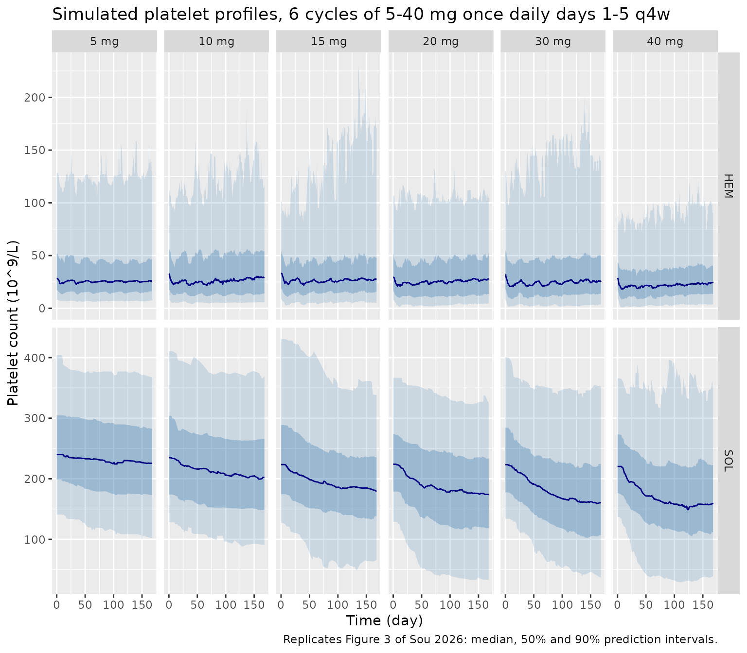
The typical SOL patient’s maturation time (844 h, 35 days) is much longer than the HEM value (142 h, 6 days). Its nadir comes much later and is shallower, consistent with the paper’s statement that HEM platelet levels are “more responsive to drug effect … and a less delayed recovery time”.
Replicate published figures
pi_summary <- function(d) {
  d |>
    summarise(
      Q05 = quantile(PLT, 0.05),
      Q25 = quantile(PLT, 0.25),
      Q50 = median(PLT),
      Q75 = quantile(PLT, 0.75),
      Q95 = quantile(PLT, 0.95),
      .groups = "drop"
    )
}

sim |>
  group_by(population, dose, time) |>
  pi_summary() |>
  mutate(dose = factor(paste(dose, "mg"), levels = paste(doses, "mg"))) |>
  ggplot(aes(time / 24, Q50)) +
  geom_ribbon(aes(ymin = Q05, ymax = Q95), alpha = 0.2, fill = "steelblue") +
  geom_ribbon(aes(ymin = Q25, ymax = Q75), alpha = 0.35, fill = "steelblue") +
  geom_line(colour = "navy") +
  facet_grid(population ~ dose, scales = "free_y") +
  labs(
    x = "Time (day)", y = "Platelet count (10^9/L)",
    title = "Simulated platelet profiles, 6 cycles of 5-40 mg once daily days 1-5 q4w",
    caption = "Replicates Figure 3 of Sou 2026: median, 50% and 90% prediction intervals."
  )
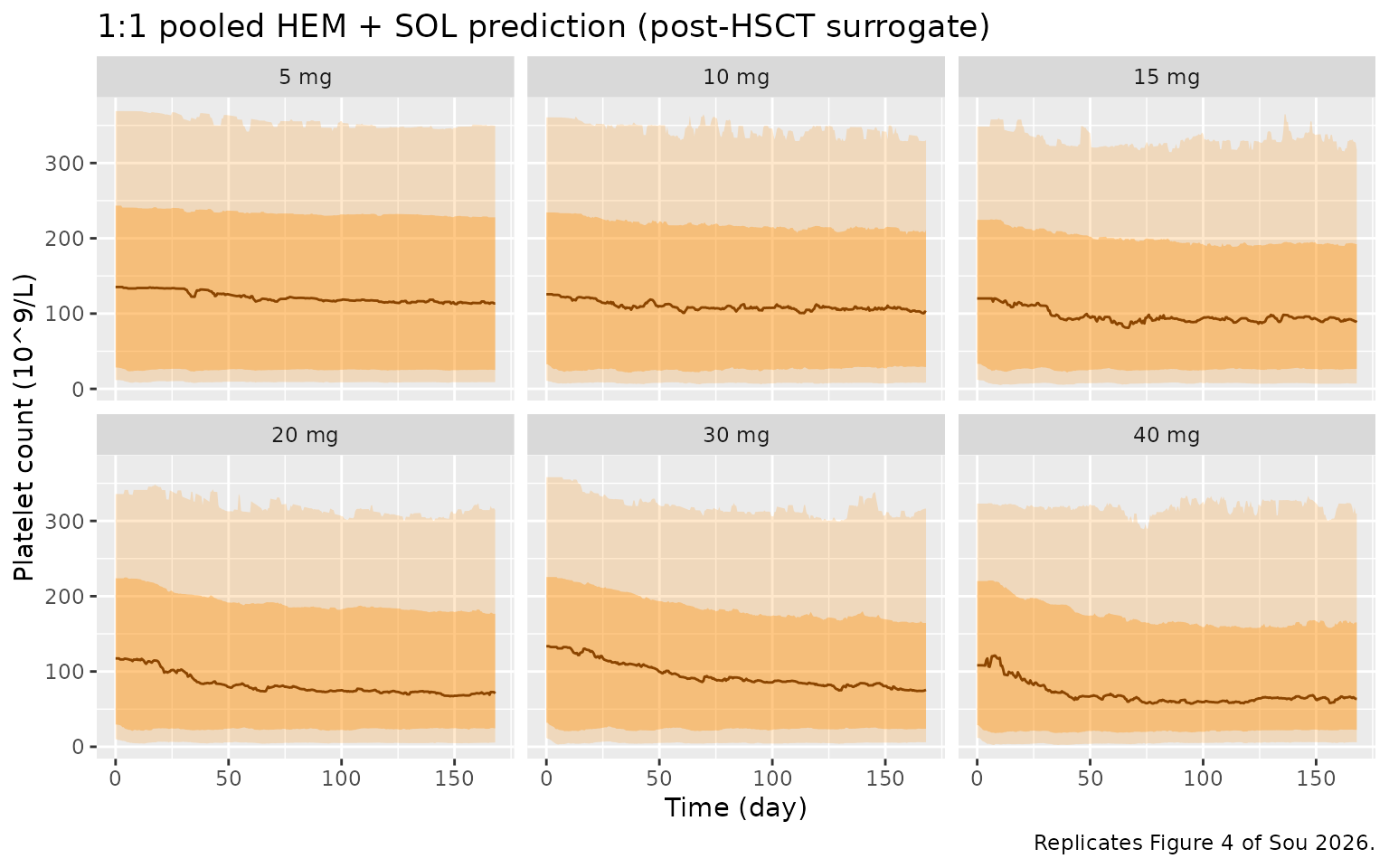
# Post-HSCT patients are represented by pooling HEM and SOL predictions 1:1.
sim |>
  group_by(dose, time) |>
  pi_summary() |>
  mutate(dose = factor(paste(dose, "mg"), levels = paste(doses, "mg"))) |>
  ggplot(aes(time / 24, Q50)) +
  geom_ribbon(aes(ymin = Q05, ymax = Q95), alpha = 0.2, fill = "darkorange") +
  geom_ribbon(aes(ymin = Q25, ymax = Q75), alpha = 0.35, fill = "darkorange") +
  geom_line(colour = "darkorange4") +
  facet_wrap(~dose, nrow = 2) +
  labs(
    x = "Time (day)", y = "Platelet count (10^9/L)",
    title = "1:1 pooled HEM + SOL prediction (post-HSCT surrogate)",
    caption = "Replicates Figure 4 of Sou 2026."
  )
sim |>
  filter(dose == 30) |>
  group_by(time) |>
  pi_summary() |>
  ggplot(aes(time / 24, Q50)) +
  geom_ribbon(aes(ymin = Q05, ymax = Q95), alpha = 0.2, fill = "darkorange") +
  geom_ribbon(aes(ymin = Q25, ymax = Q75), alpha = 0.35, fill = "darkorange") +
  geom_line(colour = "darkorange4") +
  geom_hline(yintercept = 171, linetype = "dashed") +
  labs(
    x = "Time (day)", y = "Platelet count (10^9/L)",
    title = "30 mg once daily days 1-5 q4w, 1:1 pooled prediction",
    caption = paste(
      "Simulated part of Figure 5 of Sou 2026 (the observed post-HSCT data are not public).",
      "Dashed line: observed median baseline platelet count of the 8 post-HSCT patients (171 10^9/L)."
    )
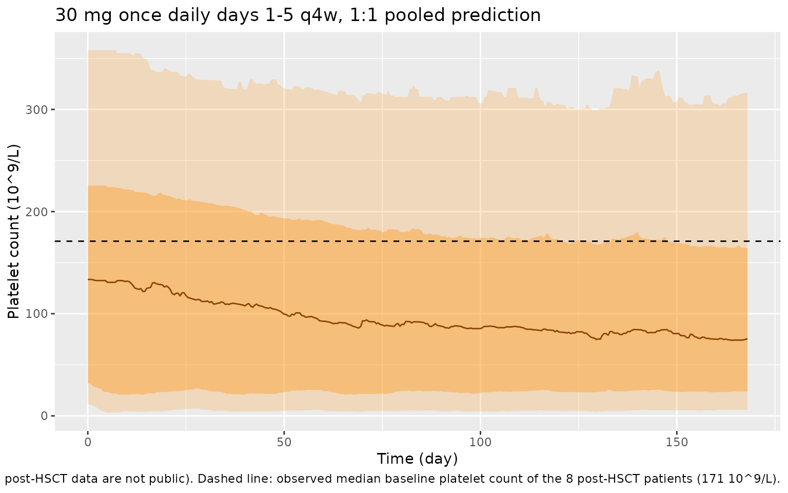
  )
Probability of thrombocytopenia (Tables 2-4)
The paper defines thrombocytopenia as at least one predicted platelet count below the CTCAE grade threshold (grade 1 < 100, grade 2 < 75, grade 3 < 50, grade 4 < 25 10^9/L) during the 6 cycles. Because siremadlin only lowers platelet counts, a HEM patient whose baseline is already below 100 stays below it after the first dose and so has a grade 1 event. That is why the HEM grade-1 probability is about 0.97 at every dose. Table 4 (post-HSCT) is the 1:1 average of the HEM and SOL arms.
thresholds <- c(G1 = 100, G2 = 75, G3 = 50, G4 = 25)
subject_min <- sim |>
  group_by(id, population, dose) |>
  summarise(
    plt_min = min(PLT),
    plt_min_post = min(PLT[time > 0]),
    .groups = "drop"
  )
# Subject-grade cells whose classification would change if time 0 were
# excluded from the window.
n_baseline_only <- sum(vapply(
  thresholds,
  function(th) sum((subject_min$plt_min < th) != (subject_min$plt_min_post < th)),
  numeric(1)
))

prob_sim <- subject_min |>
  group_by(population, dose) |>
  summarise(
    G1 = mean(plt_min < thresholds[["G1"]]),
    G2 = mean(plt_min < thresholds[["G2"]]),
    G3 = mean(plt_min < thresholds[["G3"]]),
    G4 = mean(plt_min < thresholds[["G4"]]),
    .groups = "drop"
  )
prob_sim <- bind_rows(
  prob_sim,
  prob_sim |>
    group_by(dose) |>
    summarise(across(G1:G4, mean), .groups = "drop") |>
    mutate(population = "post-HSCT (1:1)")
)

published <- tibble::tribble(
  ~population, ~dose, ~G1, ~G2, ~G3, ~G4,
  "HEM", 5, 0.970, 0.933, 0.817, 0.545,
  "HEM", 10, 0.976, 0.951, 0.846, 0.618,
  "HEM", 15, 0.980, 0.963, 0.874, 0.677,
  "HEM", 20, 0.982, 0.970, 0.898, 0.709,
  "HEM", 30, 0.980, 0.970, 0.921, 0.740,
  "HEM", 40, 0.986, 0.980, 0.939, 0.803,
  "SOL", 5, 0.041, 0.012, 0.004, 0.000,
  "SOL", 10, 0.106, 0.057, 0.028, 0.002,
  "SOL", 15, 0.169, 0.102, 0.051, 0.022,
  "SOL", 20, 0.232, 0.152, 0.079, 0.035,
  "SOL", 30, 0.333, 0.236, 0.163, 0.067,
  "SOL", 40, 0.392, 0.303, 0.220, 0.114,
  "post-HSCT (1:1)", 5, 0.498, 0.465, 0.404, 0.268,
  "post-HSCT (1:1)", 10, 0.534, 0.497, 0.430, 0.305,
  "post-HSCT (1:1)", 15, 0.568, 0.526, 0.456, 0.344,
  "post-HSCT (1:1)", 20, 0.601, 0.554, 0.482, 0.367,
  "post-HSCT (1:1)", 30, 0.651, 0.597, 0.536, 0.398,
  "post-HSCT (1:1)", 40, 0.684, 0.636, 0.574, 0.453
)

cmp <- inner_join(
  pivot_longer(prob_sim, G1:G4, names_to = "grade", values_to = "simulated"),
  pivot_longer(published, G1:G4, names_to = "grade", values_to = "published"),
  by = c("population", "dose", "grade")
) |>
  mutate(diff = simulated - published)
stopifnot(nrow(cmp) == 72)

cmp |>
  mutate(cell = sprintf("%.3f (%.3f)", simulated, published)) |>
  select(population, dose, grade, cell) |>
  pivot_wider(names_from = grade, values_from = cell) |>
  rename(
    "Population" = population,
    "Dose (mg)" = dose,
    "Grade >= 1" = G1,
    "Grade >= 2" = G2,
    "Grade >= 3" = G3,
    "Grade >= 4" = G4
  ) |>
knitr::kable(caption = "Simulated (published) probability of at least one thrombocytopenia event over 6 cycles. Published values: Tables 2, 3 and 4 of Sou 2026.")| Population | Dose (mg) | Grade >= 1 | Grade >= 2 | Grade >= 3 | Grade >= 4 |
|---|---|---|---|---|---|
| HEM | 5 | 0.960 (0.970) | 0.935 (0.933) | 0.855 (0.817) | 0.620 (0.545) |
| HEM | 10 | 0.980 (0.976) | 0.935 (0.951) | 0.870 (0.846) | 0.680 (0.618) |
| HEM | 15 | 0.980 (0.980) | 0.955 (0.963) | 0.895 (0.874) | 0.690 (0.677) |
| HEM | 20 | 0.990 (0.982) | 0.960 (0.970) | 0.920 (0.898) | 0.765 (0.709) |
| HEM | 30 | 0.985 (0.980) | 0.960 (0.970) | 0.915 (0.921) | 0.770 (0.740) |
| HEM | 40 | 0.995 (0.986) | 0.985 (0.980) | 0.955 (0.939) | 0.865 (0.803) |
| SOL | 5 | 0.060 (0.041) | 0.035 (0.012) | 0.020 (0.004) | 0.010 (0.000) |
| SOL | 10 | 0.085 (0.106) | 0.045 (0.057) | 0.015 (0.028) | 0.000 (0.002) |
| SOL | 15 | 0.170 (0.169) | 0.095 (0.102) | 0.075 (0.051) | 0.030 (0.022) |
| SOL | 20 | 0.260 (0.232) | 0.205 (0.152) | 0.115 (0.079) | 0.060 (0.035) |
| SOL | 30 | 0.295 (0.333) | 0.170 (0.236) | 0.095 (0.163) | 0.055 (0.067) |
| SOL | 40 | 0.325 (0.392) | 0.225 (0.303) | 0.155 (0.220) | 0.075 (0.114) |
| post-HSCT (1:1) | 5 | 0.510 (0.498) | 0.485 (0.465) | 0.438 (0.404) | 0.315 (0.268) |
| post-HSCT (1:1) | 10 | 0.532 (0.534) | 0.490 (0.497) | 0.443 (0.430) | 0.340 (0.305) |
| post-HSCT (1:1) | 15 | 0.575 (0.568) | 0.525 (0.526) | 0.485 (0.456) | 0.360 (0.344) |
| post-HSCT (1:1) | 20 | 0.625 (0.601) | 0.583 (0.554) | 0.518 (0.482) | 0.412 (0.367) |
| post-HSCT (1:1) | 30 | 0.640 (0.651) | 0.565 (0.597) | 0.505 (0.536) | 0.413 (0.398) |
| post-HSCT (1:1) | 40 | 0.660 (0.684) | 0.605 (0.636) | 0.555 (0.574) | 0.470 (0.453) |
With 200 subjects per arm the Monte-Carlo standard error of a probability near 0.5 is about 0.035, and the paper’s own 1000-subject simulation carries similar noise. The check therefore uses the centre and a robust quantile of the 72 differences rather than the worst cell:
summary(abs(cmp$diff))
#>    Min. 1st Qu.  Median    Mean 3rd Qu.    Max.
#> 0.00000 0.01000 0.01950 0.02469 0.03388 0.07800
stopifnot(
  # A mis-transcribed baseline, maturation time or slope shifts whole rows
  # by tens of percentage points.
  median(abs(cmp$diff)) < 0.05,
  quantile(abs(cmp$diff), 0.9) < 0.12
)
Across both tables the simulated HEM grade 4 probabilities sit somewhat above Table 2 and the SOL probabilities at 30-40 mg somewhat below Table 3. The same pattern appears with 1000 subjects per arm, so it is not only Monte-Carlo noise. Plausible causes are details of the Simulx virtual population and output grid that the paper does not report: the body-weight distribution, and how densely the predicted platelet profile was sampled when looking for threshold crossings (here every 12 h). The differences are a few percentage points, much smaller than any parameter error would produce.
The external validation in the paper compares the observed grade >= 3 incidence in post-HSCT patients at 30 mg (4 of 8, 50%) with the predicted 53.6%. The pooled simulation here gives 50.5%.
PKNCA validation
Sou 2026 reports no NCA, so the PK check is internal. After a single
dose, AUC0-inf must equal Dose / (CL/F) for every subject. A single-dose
cohort (the paper’s day-1 regimen) is simulated at each dose level with
dense sampling, and PKNCA estimates are compared with each subject’s own
Dose / cl. This confirms the transit-absorption input
delivers the whole dose and that Cc is in ng/mL.
n_pk <- 100L
pk_obs <- c(seq(0, 12, by = 0.25), seq(13, 72, by = 1), seq(76, 168, by = 4))
pk_events <- bind_rows(lapply(seq_along(doses), function(i) {
  ids <- (i - 1L) * n_pk + seq_len(n_pk)
  bind_rows(
    tibble(id = ids, time = 0, amt = doses[i], evid = 1L, cmt = "depot", dvid = NA_integer_),
    tidyr::expand_grid(id = ids, time = pk_obs) |>
      mutate(amt = 0, evid = 0L, cmt = "central", dvid = 1L)
  ) |>
    mutate(WT = 70, DIS_HEME_MALIG = 0, treatment = paste(doses[i], "mg"))
})) |>
  arrange(id, time, desc(evid))

rxode2::rxSetSeed(20260227)
sim_pk <- rxode2::rxSolve(mod, events = pk_events, keep = "treatment", returnType = "data.frame")
sim_nca <- sim_pk |>
  filter(!is.na(Cc)) |>
  select(id, time, Cc, treatment)
sim_nca <- bind_rows(
  sim_nca,
  sim_nca |> distinct(id, treatment) |> mutate(time = 0, Cc = 0)
) |>
  distinct(id, treatment, time, .keep_all = TRUE) |>
  arrange(id, treatment, time)

conc_obj <- PKNCA::PKNCAconc(sim_nca, Cc ~ time | treatment + id)
dose_df <- pk_events |>
  filter(evid == 1) |>
  select(id, time, amt, treatment)
dose_obj <- PKNCA::PKNCAdose(dose_df, amt ~ time | treatment + id)
intervals <- data.frame(
  start = 0, end = Inf,
  cmax = TRUE, tmax = TRUE, aucinf.obs = TRUE, half.life = TRUE
)
nca_res <- PKNCA::pk.nca(PKNCA::PKNCAdata(conc_obj, dose_obj, intervals = intervals))

nca_tbl <- as.data.frame(nca_res$result) |>
  filter(PPTESTCD %in% c("cmax", "tmax", "aucinf.obs", "half.life")) |>
  group_by(treatment, PPTESTCD) |>
  summarise(median = median(PPORRES, na.rm = TRUE), .groups = "drop") |>
  pivot_wider(names_from = PPTESTCD, values_from = median) |>
  mutate(treatment = factor(treatment, levels = paste(doses, "mg"))) |>
  arrange(treatment)
nca_tbl |>
  rename(
    "Dose" = treatment,
    "Cmax (ng/mL)" = cmax,
    "Tmax (h)" = tmax,
    "AUC0-inf (ng*h/mL)" = aucinf.obs,
    "t1/2 (h)" = half.life
  ) |>
knitr::kable(digits = 2, caption = "Median single-dose NCA by dose (simulated, 100 subjects per dose).")| Dose | AUC0-inf (ng*h/mL) | Cmax (ng/mL) | t1/2 (h) | Tmax (h) |
|---|---|---|---|---|
| 5 mg | 852.81 | 39.01 | 14.66 | 2.50 |
| 10 mg | 1736.56 | 78.53 | 13.33 | 2.50 |
| 15 mg | 2672.64 | 120.60 | 13.96 | 2.50 |
| 20 mg | 3058.72 | 141.41 | 12.44 | 2.50 |
| 30 mg | 4996.74 | 217.39 | 14.33 | 2.75 |
| 40 mg | 6680.09 | 318.59 | 13.78 | 2.50 |
cl_i <- sim_pk |> distinct(id, cl)
auc_ratio <- as.data.frame(nca_res$result) |>
  filter(PPTESTCD == "aucinf.obs") |>
  mutate(id = as.integer(id)) |>
  left_join(cl_i, by = "id") |>
  left_join(dose_df |> select(id, amt), by = "id") |>
  mutate(ratio = PPORRES / (1000 * amt / cl))
summary(auc_ratio$ratio)
#>    Min. 1st Qu.  Median    Mean 3rd Qu.    Max.
#>  0.9997  1.0000  1.0000  1.0000  1.0000  1.0076
stopifnot(
  abs(median(auc_ratio$ratio) - 1) < 0.02,
  quantile(abs(auc_ratio$ratio - 1), 0.9) < 0.05
)
The typical single-dose half-life, log(2) x 115 / 5.9 = 13.5 h, is close to the median PKNCA half-lives above.
Assumptions and deviations
-
IIV scale. Table 1 gives inter-individual
variability “in SD scale” (Monolix omega). Each value was squared to
give the variance used in
ini(), and all parameters were taken as log-normal, Monolix’s default. The V-CL correlation (0.631) was converted to a covariance with the two SDs. -
Body-weight reference. The covariate is Monolix
‘tBWKG’, a transformed body weight. The paper states neither the
transformation nor the reference weight. The coefficient 0.883 is
encoded as a power exponent on
WT / 70, i.e.log(WT / 70)centring with a 70 kg reference. The simulations hold weight at 70 kg because no weight distribution is published. -
Residual error form. The PK error has an additive
(
a1) and a proportional (b1) component, but the paper does not say which Monolix combined form was used. It is encoded ascombined1(SD = a + b x f), Monolix’s default combined model. This matters only for simulated observations with residual error; every check in this article uses the individual predictions. -
Concentration units. Table 1 gives the additive PK
error in ng/mL, so the fitted concentrations, and therefore
CcinEdrug = SLP x Cc, are in ng/mL. HenceCc = 1000 x central / vc(dose in mg, V/F in L), and the slope has units mL/ng. Read against mg/L instead, the drug effect would be 1000-fold too small to produce the thrombocytopenia in Tables 2 and 3. - V/F unit typo. Table 1 prints the V/F unit as ‘L/h’; it is a volume in L.
-
Transit absorption. Monolix
pkmodel(Ktr, Mtt, ka, V, Cl)uses the Savic transit model withnn = Mtt x Ktr - 1(non-integer) transit compartments ahead of a first-order absorption compartment. It is written in the integrated incomplete-gamma form (gammap()), which is exact and stays bounded when IIV pushesnnbelow zero. The transit term follows the most recent dose, which is exact here because the 0.79 h mean transit time is far shorter than the 24 h dosing interval. -
Group-specific variance. PLTZ and MMTP each have a
separate typical value and a separate IIV variance for HEM and SOL
patients. Both etas are declared and
DIS_HEME_MALIGselects one, which reproduces Monolix’sif SOL==0 ... elseif SOL==1branch exactly. rxode2 warns thatetalcirc0_hemeandetalmtt_plt_hemeare not mu-referenced. That affects only estimation efficiency if the model is refitted, not simulation. -
Covariate coding. The source carries
SOL(1 = solid tumour); the model uses the canonicalDIS_HEME_MALIG = 1 - SOL, so the unsuffixed typical values are the solid-tumour ones. - Post-HSCT prediction. The paper’s post-HSCT prediction is not a separate model. It is the 1:1 pooling of HEM and SOL simulations, and it is reproduced here the same way.
- kSR uncertainty. The paper notes that kSR is poorly estimated (95% CI 4.22e-06 to 4.10e-05 1/h; IIV SD 4.8; shrinkage 86%) and was retained on mechanistic grounds. Its value is carried unchanged.
- Threshold crossings. The paper does not state whether the pre-dose baseline counts towards a thrombocytopenia event. The minimum here is taken over the whole window including time 0. In the cohort above, excluding time 0 would change 0 of the 9600 subject-by-grade classifications, because the drug starts lowering the count as soon as it is given. The predicted profile is sampled every 12 h; the paper’s sampling grid is not reported.
- Errata. EuropePMC lists no correction or comment for Sou 2026 as of 2026-11-12.