Azithromycin (Zheng 2018)
Source:vignettes/articles/Zheng_2018_azithromycin.Rmd
Zheng_2018_azithromycin.RmdModel and source
- Citation: Zheng Y, Liu S-P, Xu B-P, Shi Z-R, Wang K, Yang J-B, Huang X, Tang B-H, Chen X-K, Shi H-Y, Zhou Y, Wu Y-E, Qi H, Jacqz-Aigrain E, Shen A-D, Zhao W. Population pharmacokinetics and dosing optimization of azithromycin in children with community-acquired pneumonia. Antimicrob Agents Chemother. 2018 Aug 27;62(9):e00686-18. doi:10.1128/AAC.00686-18
- Description: Pediatric population PK model for intravenous azithromycin in children with community-acquired pneumonia (Zheng 2018). Two-compartment model with linear elimination, allometric scaling on clearance and intercompartmental clearance (exponent 0.75 fixed) and on central and peripheral volumes (exponent 1.0 fixed) with reference body weight 21.5 kg, and a binary alanine aminotransferase covariate that reduces CL by 24 percent when ALT > 40 IU/L.
- Article: https://doi.org/10.1128/AAC.00686-18
Population
Zheng 2018 enrolled 95 hospitalized pediatric patients (53 boys, 42 girls) with suspected or confirmed community-acquired pneumonia (CAP) at four Chinese centers between 2015 and 2017. All received intravenous azithromycin (Pfizer Ireland Pharmaceuticals) by syringe pump at 10 mg/kg over a 60-min infusion once daily, in addition to routine clinical care. Sampling followed an opportunistic design tied to clinically scheduled blood draws, yielding 140 plasma concentrations across the cohort. An external validation cohort of 28 additional children (age 2.0-11.0 years, weight 10.0-50.0 kg) was characterised separately and is not part of the model-building data.
Baseline characteristics reported in Zheng 2018 Table 1: age mean 6.2
years (SD 2.6; range 2.1-11.7), body weight mean 23.9 kg (SD 9.8; range
11.0-51.0), height mean 117.7 cm (SD 19.4), alanine aminotransferase
(ALT) mean 26.8 IU/L (SD 40.2; range 3.3-374.4; median 20.3), aspartate
aminotransferase mean 33.8 IU/L (SD 32.3), blood urea nitrogen mean 3.3
mmol/L (SD 1.0), and serum creatinine mean 36.0 umol/L (SD 6.8). The
same information is available programmatically via
rxode2::rxode(readModelDb("Zheng_2018_azithromycin"))$population.
Source trace
The per-parameter origin is recorded as an in-file comment next to
each ini() entry in
inst/modeldb/specificDrugs/Zheng_2018_azithromycin.R. The
table below collects them in one place for review.
| Equation / parameter | Value | Source location |
|---|---|---|
lcl (CL typical, L/h) |
log(27.8) | Zheng 2018 Table 3, theta1 |
lvc (V1 typical, L) |
log(39.5) | Zheng 2018 Table 3, theta2 |
lvp (V2 typical, L) |
log(377) | Zheng 2018 Table 3, theta3 |
lq (Q typical, L/h) |
log(55.7) | Zheng 2018 Table 3, theta4 |
e_alt_cl (log effect of ALT > 40 on CL) |
log(0.761) | Zheng 2018 Table 3, theta5 |
allo_cl (allometric exponent on CL and Q) |
fixed 0.75 | Zheng 2018 Methods ‘Covariate analysis’ |
allo_v (allometric exponent on V1 and V2) |
fixed 1.0 | Zheng 2018 Methods ‘Covariate analysis’ |
| Reference weight (kg) | 21.5 | Zheng 2018 Table 1 median; Table 3 footnote |
| ALT binarization threshold (IU/L) | 40 | Zheng 2018 Table 3 (F_liver = 1 if ALT > 40) |
etalcl (IIV variance) |
log(0.321^2 + 1) = 0.09805 | Zheng 2018 Table 3, 32.1% CV |
etalvc (IIV variance) |
log(0.849^2 + 1) = 0.54299 | Zheng 2018 Table 3, 84.9% CV |
etalq (IIV variance) |
log(0.516^2 + 1) = 0.23624 | Zheng 2018 Table 3, 51.6% CV |
expSd (residual error) |
0.057 | Zheng 2018 Table 3, 5.7% CV exponential |
| 2-compartment ODE structure | n/a | Zheng 2018 Methods ‘Model building’ (ADVAN3 TRANS4) |
| 60-min IV infusion dosing | n/a | Zheng 2018 Methods ‘Dosing regimen’ |
Virtual cohort
The simulation below builds a virtual cohort of 200 pediatric patients whose covariate distributions approximate the published baseline characteristics (Zheng 2018 Table 1). Weight and ALT are sampled from log-normal distributions matched to the cohort medians and ranges; age is informational only because the model has no age-on-PK term once weight is allometrically accommodated.
set.seed(20180627L)  # Accepted-manuscript online date 2018-06-25; offset for reproducibility.

n_subj <- 200L

# Body weight: log-normal targeting median 21.5 kg and approximate
# 5th/95th-percentile span 11-51 kg.
wt_med <- 21.5
wt_sd  <- 0.40  # log-scale SD (~ matches the reported SD/mean ratio in Table 1)
wt <- rlnorm(n_subj, meanlog = log(wt_med), sdlog = wt_sd)
wt <- pmin(pmax(wt, 11), 51)

# ALT: heavily right-skewed; sample log-normal targeting median 20 IU/L
# and clip to the reported range 3.3-374 IU/L.
alt_med <- 20.3
alt_sd  <- 0.85
alt <- rlnorm(n_subj, meanlog = log(alt_med), sdlog = alt_sd)
alt <- pmin(pmax(alt, 3.3), 374.4)

cohort <- tibble::tibble(
  id    = seq_len(n_subj),
  WT    = wt,
  ALT   = alt,
  group = ifelse(alt > 40, "ALT > 40", "ALT <= 40")
)

# Dosing: 10 mg/kg infused over 60 min once daily for 7 days.
# A 7-day window is long enough to approach the published steady state
# for azithromycin (terminal half-life on the order of 1-2 days in this
# cohort: Vss / CL ~ 19.36 / 1.23 ~ 16 h apparent terminal, with the
# distributional phase extending the apparent t1/2 several-fold).
dose_amt_per_kg <- 10        # mg/kg
infusion_dur    <- 1         # h
n_doses         <- 7L
tau             <- 24        # h between doses

# Construct an event table per subject: dose rows + observation rows.
# rxode2 expects amt and rate (mg, mg/h) and the cmt for the central
# compartment dose; here cmt = "central" because the model has no depot.
events <- cohort |>
  dplyr::rowwise() |>
  dplyr::do({
    cov_row <- .
    dose_amt <- dose_amt_per_kg * cov_row$WT
    dose_times <- seq(0, by = tau, length.out = n_doses)

    doses <- tibble::tibble(
      id    = cov_row$id,
      time  = dose_times,
      amt   = dose_amt,
      rate  = dose_amt / infusion_dur,
      evid  = 1L,
      cmt   = "central",
      WT    = cov_row$WT,
      ALT   = cov_row$ALT,
      group = cov_row$group
    )

    # Dense observation grid: every 30 min over the full 7-day window
    # to capture the infusion plateau, distribution, and terminal phases.
    obs_grid <- seq(0, by = 0.5, length.out = 24 * 2 * n_doses + 1)
    obs <- tibble::tibble(
      id    = cov_row$id,
      time  = obs_grid,
      amt   = NA_real_,
      rate  = NA_real_,
      evid  = 0L,
      cmt   = NA_character_,
      WT    = cov_row$WT,
      ALT   = cov_row$ALT,
      group = cov_row$group
    )

    dplyr::bind_rows(doses, obs) |> dplyr::arrange(time, dplyr::desc(evid))
  }) |>
  dplyr::ungroup()

stopifnot(!anyDuplicated(unique(events[, c("id", "time", "evid")])))
Simulation
mod <- readModelDb("Zheng_2018_azithromycin")

sim <- rxode2::rxSolve(
  mod,
  events = events,
  keep   = c("group", "WT", "ALT")
) |>
  as.data.frame()
#> ℹ parameter labels from comments will be replaced by 'label()'
For a deterministic typical-value replication (Figure 1 of the source paper is an observed-concentration scatter rather than a model-predicted curve, so typical-value simulation is shown here only as a sanity check), zero out the random effects:
mod_typical <- mod |> rxode2::zeroRe()
#> ℹ parameter labels from comments will be replaced by 'label()'

# Typical 21.5 kg / ALT 20 child for one dose cycle.
ev_typ <- rxode2::et(amt = 215, rate = 215, cmt = "central", evid = 1) |>
  rxode2::et(seq(0, 24, by = 0.25))
ev_typ$WT  <- 21.5
ev_typ$ALT <- 20

sim_typ <- rxode2::rxSolve(mod_typical, events = ev_typ) |> as.data.frame()
#> ℹ omega/sigma items treated as zero: 'etalcl', 'etalvc', 'etalq'
Replicate published figures
The source paper’s Figure 1 plots the observed concentrations of 95 children without a model-predicted overlay. The simulated VPC below substitutes the typical-value and variability bands that would frame such observed points; it is qualitative rather than a literal figure replication.
# VPC envelope across the 7-day window, faceted by the ALT subgroup
# (children with normal liver function vs ALT > 40 IU/L).
sim |>
  dplyr::filter(time > 0, time <= 24 * n_doses) |>
  dplyr::group_by(time, group) |>
  dplyr::summarise(
    Q05 = quantile(Cc, 0.05, na.rm = TRUE),
    Q50 = quantile(Cc, 0.50, na.rm = TRUE),
    Q95 = quantile(Cc, 0.95, na.rm = TRUE),
    .groups = "drop"
  ) |>
  ggplot(aes(time, Q50, fill = group, colour = group)) +
  geom_ribbon(aes(ymin = Q05, ymax = Q95), alpha = 0.25, colour = NA) +
  geom_line() +
  facet_wrap(~ group) +
  scale_y_log10() +
  labs(
    x = "Time (h)",
    y = "Azithromycin Cc (mg/L)",
    title = "Simulated VPC of plasma azithromycin in pediatric CAP",
    caption = "Approximates the context of Figure 1 in Zheng 2018; observed data are not redistributed."
  ) +
  theme(legend.position = "none")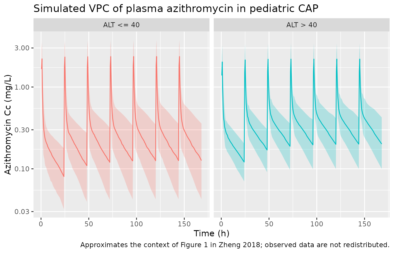
PKNCA validation
Zheng 2018 reports a population median steady-state AUC of 8.14 mgh/L for the 10 mg/kg once-daily regimen (range 3.65-18.50 mgh/L; Results ‘Model building’). The PKNCA block below computes AUC0-tau on the final dosing interval (i.e. steady state) for the simulated cohort, stratified by the ALT subgroup, so the median can be compared directly against the published value.
# Concentration data for the last dosing interval (steady state).
start_ss <- tau * (n_doses - 1)        # time of the final dose
end_ss   <- start_ss + tau

sim_nca <- sim |>
  dplyr::filter(!is.na(Cc), time >= start_ss, time <= end_ss) |>
  dplyr::select(id, time, Cc, group)

# Dose data: keep only the final-interval dose for the AUC0-tau interval.
dose_df <- events |>
  dplyr::filter(evid == 1L, time == start_ss) |>
  dplyr::select(id, time, amt, group)

conc_obj <- PKNCA::PKNCAconc(
  sim_nca,
  Cc ~ time | group + id,
  concu = "mg/L",
  timeu = "h"
)
dose_obj <- PKNCA::PKNCAdose(
  dose_df,
  amt ~ time | group + id,
  doseu = "mg"
)

intervals <- data.frame(
  start    = start_ss,
  end      = end_ss,
  cmax     = TRUE,
  tmax     = TRUE,
  cmin     = TRUE,
  auclast  = TRUE
)

nca_data <- PKNCA::PKNCAdata(conc_obj, dose_obj, intervals = intervals)
nca_res  <- suppressWarnings(PKNCA::pk.nca(nca_data))

nca_tbl <- as.data.frame(nca_res$result)
knitr::kable(
  nca_tbl |>
    dplyr::group_by(group, PPTESTCD) |>
    dplyr::summarise(
      median = median(PPORRES, na.rm = TRUE),
      p05    = quantile(PPORRES, 0.05, na.rm = TRUE),
      p95    = quantile(PPORRES, 0.95, na.rm = TRUE),
      .groups = "drop"
    ),
  digits  = 2,
  caption = "Simulated steady-state NCA parameters by ALT subgroup."
)| group | PPTESTCD | median | p05 | p95 |
|---|---|---|---|---|
| ALT <= 40 | auclast | 7.97 | 4.28 | 14.79 |
| ALT <= 40 | cmax | 2.36 | 1.31 | 3.76 |
| ALT <= 40 | cmin | 0.13 | 0.04 | 0.35 |
| ALT <= 40 | tmax | 1.00 | 1.00 | 1.00 |
| ALT > 40 | auclast | 9.56 | 6.75 | 16.42 |
| ALT > 40 | cmax | 2.20 | 1.22 | 3.43 |
| ALT > 40 | cmin | 0.20 | 0.10 | 0.42 |
| ALT > 40 | tmax | 1.00 | 1.00 | 1.00 |
Comparison against published NCA
The single quantitative NCA value reported by Zheng 2018 is the median steady-state AUC0-24 of 8.14 mg*h/L across the full cohort at 10 mg/kg (range 3.65-18.50). The cohort-level median below combines both ALT subgroups to mirror the paper’s reported median.
sim_auclast <- nca_tbl |>
  dplyr::filter(PPTESTCD == "auclast") |>
  dplyr::summarise(
    median = median(PPORRES, na.rm = TRUE),
    p05    = quantile(PPORRES, 0.05, na.rm = TRUE),
    p95    = quantile(PPORRES, 0.95, na.rm = TRUE)
  )

comparison <- tibble::tibble(
  Source     = c("Published (Zheng 2018 Results)", "Simulated (this vignette)"),
  `Median AUC0-24 ss (mg*h/L)` = c(8.14, signif(sim_auclast$median, 3)),
  `5th-95th (mg*h/L)`          = c(
    "3.65-18.50",
    sprintf("%.2f-%.2f", sim_auclast$p05, sim_auclast$p95)
  )
)

knitr::kable(comparison, caption = "Steady-state AUC0-24 comparison.")| Source | Median AUC0-24 ss (mg*h/L) | 5th-95th (mg*h/L) |
|---|---|---|
| Published (Zheng 2018 Results) | 8.14 | 3.65-18.50 |
| Simulated (this vignette) | 8.40 | 4.39-15.96 |
A side-by-side comparison of the structural-CL/Vss predictions against the paper’s reported population summaries (Results ‘Model building’):
mod_typ_ref <- mod |> rxode2::zeroRe()
#> ℹ parameter labels from comments will be replaced by 'label()'

# Closed-form typical-value predictions at the reference 21.5 kg with
# normal ALT: CL = 27.8 L/h, V1 + V2 = 39.5 + 377 = 416.5 L.
typ_pred <- tibble::tibble(
  Source     = c("Published (Zheng 2018 Results)", "Model typical values"),
  `CL/kg (L/h/kg)` = c(1.23, signif(27.8 / 21.5, 3)),
  `Vss/kg (L/kg)`  = c(19.36, signif((39.5 + 377) / 21.5, 4))
)

knitr::kable(typ_pred,
caption = "Weight-normalised CL and Vss at the 21.5 kg reference subject.")| Source | CL/kg (L/h/kg) | Vss/kg (L/kg) |
|---|---|---|
| Published (Zheng 2018 Results) | 1.23 | 19.36 |
| Model typical values | 1.29 | 19.37 |
Assumptions and deviations
- Table 3 vs Results-text discrepancy on which parameters carry IIV. Zheng 2018 Results ‘Model building’ states that interindividual variability was estimated for V1, V2, and CL, but Table 3 explicitly lists IIV percentages only for CL (32.1 percent), V1 (84.9 percent), and Q (51.6 percent) – not V2. The model file follows Table 3 (CL, V1, Q) as the authoritative parameter source; the Results prose is taken as a typographical error.
-
Table 3 equation-column typography. The Table 3
‘Final estimate’ column prints the volume and Q equations as
V1 = theta2 * (wt/21.5)^theta2,V2 = theta3 * (wt/21.5)^theta3, andQ = theta4 * (wt/21.5)^0.75 theta4. These are typesetting artifacts; the Methods ‘Covariate analysis’ section states explicitly that the a priori allometric coefficient was 0.75 for clearances and 1 for volumes, which is what the model implements. -
Residual error encoded as log-normal
(
lnorm). Zheng 2018 reports an exponential residual model with 5.7 percent CV (Table 3) and very high RSE (161.6 percent), implying the residual is poorly identified. The model encodes the value asexpSd = 0.057on thelnormresidual which is the rxode2/nlmixr2 equivalent of NONMEMY = IPRED * exp(EPS). Users who prefer a proportional approximation can substituteCc ~ prop(propSd)withpropSd = 0.057; the two forms are numerically very close at this magnitude. - Virtual-cohort distributions are illustrative. The vignette samples weight from a log-normal centered on the reported median 21.5 kg with spread chosen to roughly span 11-51 kg, and ALT from a log-normal centered on the reported median 20.3 IU/L with spread chosen to roughly span the reported 3.3-374 IU/L range. The original per-subject covariate dataset is not publicly available; downstream users should overwrite the cohort with their own covariates when running site-specific simulations.
- No model-predicted figure to replicate. Figure 1 of the source paper plots observed concentrations from 95 children with no model overlay; the VPC chunk here is qualitative context rather than a literal replication. Figure 2 shows Monte Carlo target attainment as a function of dose and ALT subgroup; the optimal-dosing simulation logic is summarised in the paper’s Results ‘Simulation and dosing regimen optimization’ but the full Monte Carlo apparatus is out of scope for this vignette.
- Supplemental file not required for parameter sourcing. Zheng 2018 Supplemental File 1 (PDF, 0.2 MB) contains the goodness-of-fit, CWRES, and NPDE diagnostic plots referenced in Results ‘Model qualification’. It does not carry numerical parameter values beyond what Table 3 reports, so it is not needed to build the model file.