Pemetrexed clearance and renal biomarkers (de Rouw 2024)
Source:vignettes/articles/deRouw_2024_pemetrexed.Rmd
deRouw_2024_pemetrexed.RmdModel and source
de Rouw 2024 fits a three-compartment population PK model for intravenous pemetrexed to 66 patients with lung cancer and compares six renal-function biomarkers as covariates on clearance: the CKD-EPI equation with creatinine, with cystatin C, and with both; plasma pro-enkephalin (PENK) alone; the PENK-creatinine eGFR of Beunders et al.; and cystatin C combined with PENK. Each covariate model is packaged as its own model file, and all six point at this article.
| Model | Clearance equation (L/h), de Rouw 2024 Table 2 | IIV CL (Table 3) | dOFV |
|---|---|---|---|
deRouw_2024_pemetrexed_ckdepicr |
1.66 + 0.0358 x CKD-EPI creatinine | 16.2% | -38.1 |
deRouw_2024_pemetrexed_ckdepicys |
2.46 + 0.0344 x CKD-EPI cystatin C | 17.6% | -29.2 |
deRouw_2024_pemetrexed_ckdepicrcys |
1.89 + 0.038 x CKD-EPI creatinine-cystatin C | 16.1% | -49.5 |
deRouw_2024_pemetrexed_penk |
5.62 x exp(-0.0877 x PENK / 35) | 21.8% | -13.0 |
deRouw_2024_pemetrexed_egfrpenkcr |
1.82 + 0.0295 x eGFR-PENK-creatinine | 18.1% | -32.8 |
deRouw_2024_pemetrexed_ckdepicyspenk |
5.81 x exp(-0.0206 x PENK / 35) x (CKD-EPI cystatin C / 75)^0.378 | 17.3% | -41.0 |
All eGFR values are in mL/min, de-indexed to the patient’s body
surface area (CRCL column, NOT mL/min/1.73 m^2); PENK is in
pmol/L (PROENKEPHALIN column). The combined
creatinine-cystatin C model fitted best.
The paper reports only these clearance equations and the IIV on clearance. The model it refits, “a previously developed three-compartment pharmacokinetic model without covariates”, is the de Rouw 2021 base model (doi:10.1007/s40262-020-00972-1), and the refitted volumes, intercompartmental clearances, their IIV and the residual error are not published. Those parameters are therefore carried from the de Rouw 2021 supplementary Table S1 base-model column in all six files (see Assumptions and deviations).
- Citation: de Rouw N, Beunders R, Hartmann O, Schulte J, Boosman RJ, Derijks HJ, Burger DM, van den Heuvel MM, Hilbrands LB, Pickkers P, ter Heine R. A comparison of the renal function biomarkers serum creatinine, pro-enkephalin and cystatin C to predict clearance of pemetrexed. Cancer Chemother Pharmacol. 2024;94(6):799-806. doi:10.1007/s00280-024-04717-w. Volumes, intercompartmental clearances, their IIV and the residual error: de Rouw N, Boosman RJ, Huitema ADR, Hilbrands LB, Svensson EM, Derijks HJ, van den Heuvel MM, Burger DM, ter Heine R. Rethinking the application of pemetrexed for patients with renal impairment: a pharmacokinetic analysis. Clin Pharmacokinet. 2021;60(5):649-654. doi:10.1007/s40262-020-00972-1 (Supplementary Table S1, base model).
- Article: https://doi.org/10.1007/s00280-024-04717-w (open access; PMC11573856)
mod_names <- c(
  ckdepicr = "deRouw_2024_pemetrexed_ckdepicr",
  ckdepicys = "deRouw_2024_pemetrexed_ckdepicys",
  ckdepicrcys = "deRouw_2024_pemetrexed_ckdepicrcys",
  penk = "deRouw_2024_pemetrexed_penk",
  egfrpenkcr = "deRouw_2024_pemetrexed_egfrpenkcr",
  ckdepicyspenk = "deRouw_2024_pemetrexed_ckdepicyspenk"
)
mods <- lapply(mod_names, function(nm) rxode2::rxode(readModelDb(nm)))
#> ℹ parameter labels from comments will be replaced by 'label()'
#> ℹ parameter labels from comments will be replaced by 'label()'
#> ℹ parameter labels from comments will be replaced by 'label()'
#> ℹ parameter labels from comments will be replaced by 'label()'
#> ℹ parameter labels from comments will be replaced by 'label()'
#> ℹ parameter labels from comments will be replaced by 'label()'
model_labels <- c(
  ckdepicr = "CKD-EPI CR",
  ckdepicys = "CKD-EPI CYS",
  ckdepicrcys = "CKD-EPI CR-CYS",
  penk = "PENK",
  egfrpenkcr = "eGFR PENK-CR",
  ckdepicyspenk = "PENK + CKD-EPI CYS"
)
vapply(mods, function(u) paste(u$state, collapse = " + "), character(1))
#>                              ckdepicr                             ckdepicys
#> "central + peripheral1 + peripheral2" "central + peripheral1 + peripheral2"
#>                           ckdepicrcys                                  penk
#> "central + peripheral1 + peripheral2" "central + peripheral1 + peripheral2"
#>                            egfrpenkcr                         ckdepicyspenk
#> "central + peripheral1 + peripheral2" "central + peripheral1 + peripheral2"
Population
The analysis set is 66 patients from two multicentre clinical trials (NCT03655821, NCT03656549) with paired baseline serum creatinine, serum cystatin C and plasma PENK, contributing 378 pemetrexed plasma concentrations (at least four per patient). de Rouw 2024 Table 1: 50% male, median age 65 years (IQR 59-71), weight 77.1 kg (63.7-84.8), BSA 1.9 m^2 (1.7-2.0). Renal markers, median (IQR): CKD-EPI creatinine 97.0 (85.4-104.1), CKD-EPI cystatin C 75.1 (59.8-92.2), CKD-EPI creatinine-cystatin C 89.0 (73.3-99.5) and eGFR PENK-creatinine 112.5 (98.9-122.6) mL/min; PENK 37.3 (30.8-46.1) pmol/L. Five patients had a CKD-EPI creatinine below 60 mL/min, and 19 (28.4%) were sarcopenic by fat-free mass index.
Source trace
| Element | Value | Source |
|---|---|---|
| Clearance equations, six models | see table above | de Rouw 2024 Table 2 |
| Reference values 35 pmol/L (PENK) and 75 mL/min (CKD-EPI cystatin C) | “median … in the population” | de Rouw 2024 Table 2 footnote |
IIV on CL, per model (etalcl) |
16.1-21.8% | de Rouw 2024 Table 3 |
| IIV reported as sqrt(omega^2) x 100 | 21.0% with $OMEGA 0.0442 | de Rouw 2021 supplement Table S1 and NONMEM code |
| Log-normal IIV on total CL | CL = TVCL * EXP(ETA(1)) |
de Rouw 2021 supplement NONMEM code |
V1 (lvc) |
6.70 L | de Rouw 2021 Table S1, Base |
Q1 (lq) |
6.56 L/h (printed mL/min) | de Rouw 2021 Table S1, Base |
V2 (lvp) |
8.01 L | de Rouw 2021 Table S1, Base |
Q2 (lq2) |
0.04 L/h (printed mL/min) | de Rouw 2021 Table S1, Base |
V3 (lvp2) |
1.25 L | de Rouw 2021 Table S1, Base |
| Allometric exponents 1 (V) and 0.75 (Q), reference 70 kg | fixed | de Rouw 2021 supplement section 1.1 and $PK |
| IIV V1 / V2 / V3 | 33.6 / 31.2 / 48.1% | de Rouw 2021 Table S1, Base |
| Correlations V1-V2 / V1-V3 / V2-V3 | 32.5 / 63.1 / 61.9% | de Rouw 2021 Table S1, Base |
Proportional residual error (propSd) |
23.5% | de Rouw 2021 Table S1, Base |
| Three-compartment structure, 10-min infusion | ADVAN5, D1 = 0.16667 h | de Rouw 2021 supplement NONMEM code |
Typical clearance at the cohort medians
The clearance the model computes for a typical patient must equal the
printed Table 2 equation evaluated at the same covariates. The check
below solves each model with the random effects zeroed at the Table 1
medians and compares the model’s cl with the closed form;
both sides use the same parameters, so the tolerance is tight.
clpred <- function(model, CRCL, PROENKEPHALIN) {
  switch(model,
    ckdepicr = 1.66 + 0.0358 * CRCL,
    ckdepicys = 2.46 + 0.0344 * CRCL,
    ckdepicrcys = 1.89 + 0.038 * CRCL,
    penk = 5.62 * exp(-0.0877 * PROENKEPHALIN / 35),
    egfrpenkcr = 1.82 + 0.0295 * CRCL,
    ckdepicyspenk = 5.81 * exp(-0.0206 * PROENKEPHALIN / 35) * (CRCL / 75)^0.378
  )
}
# Table 1 medians of the renal marker each model's CRCL column carries.
crcl_median <- c(
  ckdepicr = 97.0, ckdepicys = 75.1, ckdepicrcys = 89.0,
  penk = NA, egfrpenkcr = 112.5, ckdepicyspenk = 75.1
)
penk_median <- 37.3
dose_mg <- 500 * 1.9 # 500 mg/m^2 at the Table 1 median BSA
obs_times <- c(
  0, 1 / 6, 0.25, 0.5, 0.75, 1, 1.5, 2, 3, 4, 6, 8, 12, 16, 24, 36, 48,
  72, 96, 120, 168
)
typ_events <- function(model) {
  rxode2::et(amt = dose_mg, dur = 1 / 6, cmt = "central") |>
    rxode2::et(obs_times, cmt = "central") |>
    as.data.frame() |>
    mutate(
      id = 1L,
      WT = 77.1,
      CRCL = ifelse(is.na(crcl_median[[model]]), 90, crcl_median[[model]]),
      PROENKEPHALIN = penk_median
    )
}
typ <- bind_rows(lapply(names(mods), function(m) {
  sim <- rxode2::rxSolve(rxode2::zeroRe(mods[[m]]), events = typ_events(m))
  as.data.frame(sim) |> mutate(model = m)
}))
#> ℹ omega/sigma items treated as zero: 'etalcl', 'etalvc', 'etalvp', 'etalvp2'
#> ℹ omega/sigma items treated as zero: 'etalcl', 'etalvc', 'etalvp', 'etalvp2'
#> ℹ omega/sigma items treated as zero: 'etalcl', 'etalvc', 'etalvp', 'etalvp2'
#> ℹ omega/sigma items treated as zero: 'etalcl', 'etalvc', 'etalvp', 'etalvp2'
#> ℹ omega/sigma items treated as zero: 'etalcl', 'etalvc', 'etalvp', 'etalvp2'
#> ℹ omega/sigma items treated as zero: 'etalcl', 'etalvc', 'etalvp', 'etalvp2'
typ_cl <- typ |>
  group_by(model) |>
  summarise(cl_model = first(cl), CRCL = first(CRCL), PROENKEPHALIN = first(PROENKEPHALIN)) |>
  rowwise() |>
  mutate(cl_printed = clpred(model, CRCL, PROENKEPHALIN)) |>
  ungroup() |>
  mutate(model = factor(model, levels = names(mods))) |>
  arrange(model)
stopifnot(all(abs(typ_cl$cl_model / typ_cl$cl_printed - 1) < 1e-6))
typ_cl |>
  mutate(
    model = model_labels[as.character(model)],
    CRCL = ifelse(model == "PENK", NA, CRCL)
  ) |>
  rename(
    "Covariate model" = model,
    "eGFR (mL/min)" = CRCL,
    "PENK (pmol/L)" = PROENKEPHALIN,
    "Model CL (L/h)" = cl_model,
    "Table 2 CL (L/h)" = cl_printed
  ) |>
knitr::kable(digits = 3, caption = "Typical clearance at the de Rouw 2024 Table 1 medians.")| Covariate model | Model CL (L/h) | eGFR (mL/min) | PENK (pmol/L) | Table 2 CL (L/h) |
|---|---|---|---|---|
| CKD-EPI CR | 5.133 | 97.0 | NA | 5.133 |
| CKD-EPI CYS | 5.043 | 75.1 | NA | 5.043 |
| CKD-EPI CR-CYS | 5.272 | 89.0 | NA | 5.272 |
| PENK | 5.119 | NA | 37.3 | 5.119 |
| eGFR PENK-CR | 5.139 | 112.5 | NA | 5.139 |
| PENK + CKD-EPI CYS | 5.687 | 75.1 | 37.3 | 5.687 |
Five of the six models give a typical clearance of 5.1-5.3 L/h at the cohort medians. The cystatin C + PENK model gives 5.7 L/h, about 10% higher; that is what its Table 2 equation evaluates to as printed (see Assumptions and deviations).
Typical concentration-time profiles
ggplot(
  typ |> filter(time > 0),
  aes(time, Cc, colour = model_labels[model])
) +
  geom_line() +
  scale_y_log10() +
  coord_cartesian(xlim = c(0, 48)) +
  labs(x = "Time after start of infusion (h)", y = "Pemetrexed (mg/L)", colour = NULL)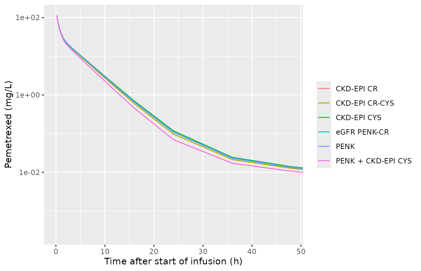
Typical pemetrexed concentration-time profiles after a 950 mg (500 mg/m^2) 10-min infusion, each model at the Table 1 medians.
Virtual cohort
Each renal marker is drawn log-normally from its Table 1 median and IQR (log-SD = log(Q3/Q1) / 1.349). The paper does not report the joint distribution, so the eGFR markers share a common latent renal-function score (correlation 0.64 between any two) and PENK runs opposite to it. Weight is drawn the same way from its Table 1 median and IQR. 150 virtual patients are simulated with each model.
rxode2::rxSetSeed(20241105)
n_sub <- 150
lsd <- function(q1, q3) log(q3 / q1) / 1.349
z_renal <- rnorm(n_sub)
draw <- function(median, q1, q3, sign = 1) {
  median * exp(lsd(q1, q3) * (sign * 0.8 * z_renal + 0.6 * rnorm(n_sub)))
}
cohort <- tibble(
  id = seq_len(n_sub),
  WT = 77.1 * exp(lsd(63.7, 84.8) * rnorm(n_sub)),
  egfr_cr = draw(97.0, 85.4, 104.1),
  egfr_cys = draw(75.1, 59.8, 92.2),
  egfr_crcys = draw(89.0, 73.3, 99.5),
  egfr_penkcr = draw(112.5, 98.9, 122.6),
  PROENKEPHALIN = draw(37.3, 30.8, 46.1, sign = -1)
)
crcl_column <- c(
  ckdepicr = "egfr_cr", ckdepicys = "egfr_cys", ckdepicrcys = "egfr_crcys",
  penk = "egfr_cr", egfrpenkcr = "egfr_penkcr", ckdepicyspenk = "egfr_cys"
)
summary(select(cohort, -id))
#>        WT            egfr_cr          egfr_cys        egfr_crcys
#>  Min.   : 45.89   Min.   : 68.22   Min.   : 39.40   Min.   : 50.69
#>  1st Qu.: 65.36   1st Qu.: 88.98   1st Qu.: 61.44   1st Qu.: 76.67
#>  Median : 77.93   Median : 97.09   Median : 76.66   Median : 89.21
#>  Mean   : 79.87   Mean   : 99.35   Mean   : 79.14   Mean   : 90.49
#>  3rd Qu.: 91.08   3rd Qu.:108.93   3rd Qu.: 91.54   3rd Qu.:102.76
#>  Max.   :135.22   Max.   :156.12   Max.   :175.63   Max.   :154.47
#>   egfr_penkcr     PROENKEPHALIN
#>  Min.   : 76.84   Min.   :15.63
#>  1st Qu.:102.53   1st Qu.:29.58
#>  Median :111.61   Median :37.32
#>  Mean   :115.18   Mean   :38.39
#>  3rd Qu.:128.77   3rd Qu.:44.19
#>  Max.   :165.44   Max.   :93.05
cohort_events <- function(model) {
  cov <- cohort |>
    mutate(CRCL = .data[[crcl_column[[model]]]]) |>
    select(id, WT, CRCL, PROENKEPHALIN)
  rxode2::et(amt = dose_mg, dur = 1 / 6, cmt = "central") |>
    rxode2::et(obs_times, cmt = "central") |>
    rxode2::et(id = cov$id) |>
    as.data.frame() |>
    left_join(cov, by = "id")
}
sim <- bind_rows(lapply(names(mods), function(m) {
  as.data.frame(rxode2::rxSolve(mods[[m]], events = cohort_events(m))) |>
    mutate(model = m)
}))
Replicate Figure 1: true versus predicted clearance
de Rouw 2024 Figure 1 plots each patient’s empirical Bayes clearance (“CLtrue”) against the Table 2 prediction (“CLpred”). The analogue here plots each virtual patient’s individual clearance (with IIV) against the Table 2 equation evaluated at that patient’s covariates.
cl_ind <- sim |>
  group_by(model, id) |>
  summarise(cl_true = first(cl), CRCL = first(CRCL), PROENKEPHALIN = first(PROENKEPHALIN), .groups = "drop") |>
  rowwise() |>
  mutate(cl_pred = clpred(model, CRCL, PROENKEPHALIN)) |>
  ungroup() |>
  mutate(panel = factor(model_labels[model], levels = model_labels))
ggplot(cl_ind, aes(cl_pred, cl_true)) +
  geom_point(size = 0.8) +
  geom_abline(slope = 1, intercept = 0) +
  facet_wrap(~panel, ncol = 2) +
  coord_equal(xlim = c(0, 9), ylim = c(0, 9)) +
  labs(x = "CLpred (L/h)", y = "CLtrue (L/h)")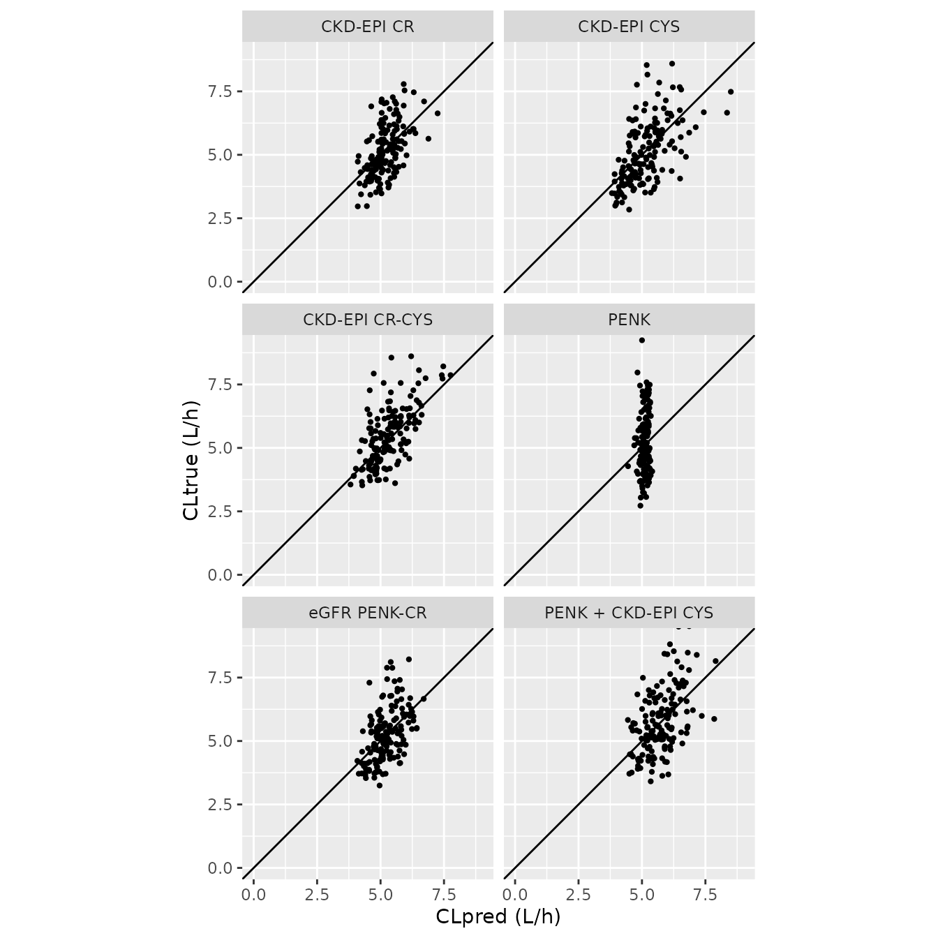
Replicates Figure 1 of de Rouw 2024: individual versus covariate-predicted clearance for the six covariate models, with the line of unity.
fig1_check <- cl_ind |>
  group_by(model) |>
  summarise(
    median_ratio = median(cl_true / cl_pred),
    sd_log_ratio = sd(log(cl_true / cl_pred))
  )
fig1_check
#> # A tibble: 6 × 3
#>   model         median_ratio sd_log_ratio
#>   <chr>                <dbl>        <dbl>
#> 1 ckdepicr             0.979        0.172
#> 2 ckdepicrcys          1.01         0.165
#> 3 ckdepicys            0.967        0.195
#> 4 ckdepicyspenk        0.992        0.192
#> 5 egfrpenkcr           0.980        0.172
#> 6 penk                 0.999        0.224
# The IIV is log-normal around the Table 2 prediction, so the median ratio
# sits at 1 and the SD of the log-ratio near the Table 3 IIV (0.16-0.22).
stopifnot(
  all(abs(fig1_check$median_ratio - 1) < 0.08),
  all(fig1_check$sd_log_ratio > 0.10 & fig1_check$sd_log_ratio < 0.30)
)
As in the paper’s Figure 1, the PENK model compresses CLpred into a narrow band: over the cohort’s PENK range, exp(-0.0877 x PENK / 35) varies by only a few percent, so nearly all of the between-patient spread is left to the IIV.
Visual predictive check (best model)
vpc <- sim |>
  filter(model == "ckdepicrcys", time > 0) |>
  group_by(time) |>
  summarise(
    p05 = quantile(Cc, 0.05),
    p50 = median(Cc),
    p95 = quantile(Cc, 0.95)
  )
ggplot(vpc, aes(time)) +
  geom_ribbon(aes(ymin = p05, ymax = p95), alpha = 0.25) +
  geom_line(aes(y = p50)) +
  scale_y_log10() +
  coord_cartesian(xlim = c(0, 48)) +
  labs(x = "Time after start of infusion (h)", y = "Pemetrexed (mg/L)")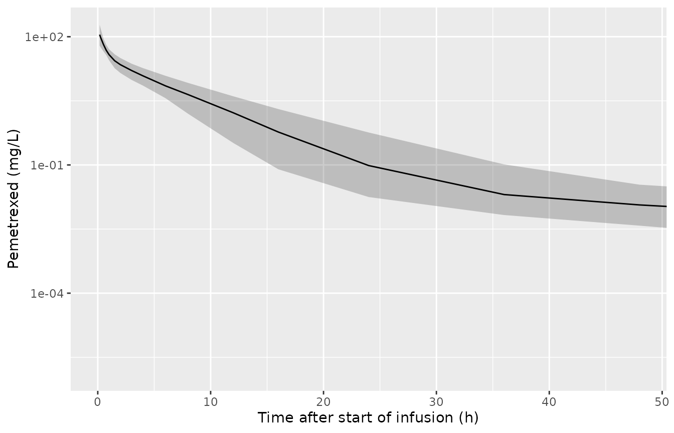
Simulated 5th, 50th and 95th percentiles of pemetrexed concentration for the CKD-EPI creatinine-cystatin C model (950 mg over 10 min).
PKNCA validation
For a linear model, AUC0-inf after an intravenous dose is exactly Dose / CL. PKNCA’s AUC0-inf on the typical-value profiles is therefore compared with Dose / CL from the Table 2 equation; the two sides share parameters, so any difference is integration and extrapolation error.
conc_typ <- typ |>
  filter(!is.na(Cc)) |>
  select(time, Cc, model) |>
  mutate(id = as.integer(factor(model, levels = names(mods))))
dose_typ <- conc_typ |>
  distinct(id, model) |>
  mutate(time = 0, amt = dose_mg)
nca_typ <- PKNCA::pk.nca(PKNCA::PKNCAdata(
  PKNCA::PKNCAconc(conc_typ, Cc ~ time | model + id),
  PKNCA::PKNCAdose(dose_typ, amt ~ time | model + id),
  intervals = data.frame(start = 0, end = Inf, cmax = TRUE, aucinf.obs = TRUE, half.life = TRUE)
))
sim_typ <- as.data.frame(nca_typ) |>
  filter(PPTESTCD %in% c("aucinf.obs", "cmax", "half.life")) |>
  select(model, PPTESTCD, PPORRES)
ref_typ <- typ_cl |>
  transmute(model = as.character(model), aucinf.obs = dose_mg / cl_printed)
cmp <- nlmixr2lib::ncaComparisonTable(
  simulated = sim_typ,
  reference = ref_typ,
  by = "model",
  params = "aucinf.obs",
  units = c(aucinf.obs = "mg*h/L"),
  tolerance_pct = 20
)
knitr::kable(cmp, caption = "Typical-value AUC0-inf from PKNCA versus Dose / CL from the Table 2 equation.")| NCA parameter | model | Reference | Simulated | % diff |
|---|---|---|---|---|
| AUC0-∞ (obs) (mg*h/L) | ckdepicr | 185 | 186 | +0.3% |
| AUC0-∞ (obs) (mg*h/L) | ckdepicys | 188 | 189 | +0.3% |
| AUC0-∞ (obs) (mg*h/L) | ckdepicrcys | 180 | 181 | +0.3% |
| AUC0-∞ (obs) (mg*h/L) | penk | 186 | 186 | +0.3% |
| AUC0-∞ (obs) (mg*h/L) | egfrpenkcr | 185 | 185 | +0.3% |
| AUC0-∞ (obs) (mg*h/L) | ckdepicyspenk | 167 | 167 | +0.3% |
auc_diff <- sim_typ |>
  filter(PPTESTCD == "aucinf.obs") |>
  left_join(ref_typ, by = "model") |>
  mutate(pct = 100 * (PPORRES / aucinf.obs - 1))
stopifnot(all(abs(auc_diff$pct) < 3))
conc_sim <- sim |>
  filter(!is.na(Cc)) |>
  select(id, time, Cc, model)
dose_sim <- conc_sim |>
  distinct(id, model) |>
  mutate(time = 0, amt = dose_mg)
nca_sim <- PKNCA::pk.nca(PKNCA::PKNCAdata(
  PKNCA::PKNCAconc(conc_sim, Cc ~ time | model + id),
  PKNCA::PKNCAdose(dose_sim, amt ~ time | model + id),
  intervals = data.frame(start = 0, end = Inf, cmax = TRUE, aucinf.obs = TRUE, half.life = TRUE)
))
#> Warning in assert_conc(conc, any_missing_conc = any_missing_conc): Negative
#> concentrations found
#> Warning in assert_conc(conc = conc): Negative concentrations found
#> Warning in assert_conc(conc, any_missing_conc = any_missing_conc): Negative
#> concentrations found
#> Warning in assert_conc(conc, any_missing_conc = any_missing_conc): Negative
#> concentrations found
#> Warning in assert_conc(conc, any_missing_conc = any_missing_conc): Negative
#> concentrations found
#> Warning in assert_conc(conc, any_missing_conc = any_missing_conc): Negative
#> concentrations found
#> Warning in assert_conc(conc, any_missing_conc = any_missing_conc): Negative
#> concentrations found
#> Warning in log(data$conc): NaNs produced
#> Warning in assert_conc(conc, any_missing_conc = any_missing_conc): Negative
#> concentrations found
#> Warning in log(conc.2/conc.1): NaNs produced
as.data.frame(nca_sim) |>
  filter(PPTESTCD %in% c("cmax", "aucinf.obs", "half.life")) |>
  group_by(model, PPTESTCD) |>
  summarise(median = median(PPORRES, na.rm = TRUE), .groups = "drop") |>
  pivot_wider(names_from = PPTESTCD, values_from = median) |>
  mutate(model = model_labels[model]) |>
  rename(
    "Covariate model" = model,
    "Cmax (mg/L)" = cmax,
    "AUC0-inf (mg*h/L)" = aucinf.obs,
    "Terminal t1/2 (h)" = half.life
  ) |>
knitr::kable(digits = 2, caption = "Median simulated NCA by covariate model (150 virtual patients each, 950 mg over 10 min).")| Covariate model | AUC0-inf (mg*h/L) | Cmax (mg/L) | Terminal t1/2 (h) |
|---|---|---|---|
| CKD-EPI CR | 187.42 | 112.16 | 24.76 |
| CKD-EPI CR-CYS | 177.94 | 111.75 | 22.15 |
| CKD-EPI CYS | 192.28 | 110.70 | 22.57 |
| PENK + CKD-EPI CYS | 171.42 | 111.15 | 21.53 |
| eGFR PENK-CR | 183.67 | 107.21 | 23.38 |
| PENK | 186.60 | 113.76 | 20.85 |
de Rouw 2024 reports no NCA, so the cohort table is descriptive.
Assumptions and deviations
- Volumes, intercompartmental clearances, their IIV and the residual error are carried from de Rouw 2021, not from the 2024 fit. de Rouw 2024 refitted the 2021 base model to its own 66 patients but published only the clearance equations (Table 2) and the IIV on clearance (Table 3). The carried values are the de Rouw 2021 supplementary Table S1 base-model column, estimated on a different dataset (47 patients from the manufacturer’s renal-impairment study). They shape the concentration-time curve, not the AUC, which depends only on the reported clearance.
- Q1 and Q2 are read as L/h. de Rouw 2021 Table S1 prints them in “mL/min”; 6.56 mL/min (0.39 L/h) against a central volume of 6.7 L is implausible for pemetrexed distribution, and the NONMEM code uses the values directly with clearances in L/h.
- Allometric scaling is applied to the volumes and the intercompartmental clearances only. The carried de Rouw 2021 values are 70 kg values with exponents 1 (volumes) and 0.75 (flows), and they keep that scaling here. Clearance follows the Table 2 equations as printed, which carry no weight term.
- IIV percentages are converted as omega^2 = (percent / 100)^2. The de Rouw 2021 supplement pairs its “IIV CL 21.0%” with a NONMEM omega of 0.0442 (0.210^2), and its volume IIVs and residual error follow the same convention; the 2024 Table 3 percentages are assumed to follow it too.
- The cystatin C + PENK equation is transcribed as printed. At the cohort medians it gives 5.7 L/h, about 10% above the other five models (5.1-5.3 L/h), whereas the paper reports a mean prediction error of only 1.7% for it. Its Figure 1 panel cannot settle whether a coefficient is misprinted, so the printed values are kept.
- The PENK reference is the printed 35 pmol/L, which the Table 2 footnote calls the population median, although Table 1 tabulates 37.3 pmol/L.
- Dose and infusion. de Rouw 2024 does not restate the dose; the simulations use the labelled 500 mg/m^2 at the Table 1 median BSA of 1.9 m^2 (950 mg) as a 10-min infusion, the duration in the de Rouw 2021 control stream.
-
Covariate distributions. Only medians and IQRs are
reported, so each marker is log-normal with an assumed correlation
structure (see Virtual cohort). The eGFR models do not need the other
markers; the
penkmodel ignoresCRCL.