DNDI-6148 (Assmus 2026)

Model and source

Citation: Assmus F, Adehin A, Hoglund RM, Mowbray CE, Gillon JY, Blesson S, Braillard S, Chatelain E, Scandale I, Tarning J. (2026). Population pharmacokinetics of DNDI-6148 in healthy adults. PLoS Negl Trop Dis 20(4):e0014220. doi:10.1371/journal.pntd.0014220. Final NONMEM control stream: S1 Code of that paper.
Description: One-compartment population PK model with first-order oral absorption for the benzoxaborole antileishmanial / antichagasic DNDI-6148 in healthy adult men, fitted to the first-in-human single-ascending-dose study (10-380 mg, eight cohorts, 48 subjects). The drug’s non-linear pharmacokinetics are carried by two exponential effects of the weight-normalised dose, centred on the study median of 1.7 mg/kg: one on relative oral bioavailability and one on apparent clearance. The two act in opposite directions on exposure, which is why Cmax rises less than dose-proportionally while AUCinf stays approximately dose-linear. Allometric body-weight scaling (0.75 on clearance, 1 on volume, both fixed) sits underneath. Inter-individual variability on apparent volume was estimated near zero and fixed to zero by the authors, so no eta is carried on it here. See modellib(‘Henninger_2026_dndi6148_mouse’) and modellib(‘Henninger_2026_dndi6148_human’) for the independent murine target-site PK/PD model of the same molecule and its allometric human projection; this model is the first fit to actual human data.
Article: https://doi.org/10.1371/journal.pntd.0014220
Supplement (S1 Code, the final NONMEM control stream): https://doi.org/10.1371/journal.pntd.0014220

DNDI-6148 is a benzoxaborole under development by the Drugs for Neglected Diseases initiative for visceral / cutaneous leishmaniasis and Chagas disease. This model is the first population PK analysis fitted to human data, using the first-in-human single-ascending-dose study. The package also carries an independent murine target-site PK/PD model of the same molecule (modellib("Henninger_2026_dndi6148_mouse")) and that paper’s own allometric human projection (modellib("Henninger_2026_dndi6148_human")); the three are separate fits and their parameters are not interconvertible.

Population

The analysis pooled the 48 participants who received active drug in a randomised, double-blind, placebo-controlled, single-centre Phase 1 single ascending dose study (EudraCT 2018-004023-37; ISRCTN54981564) run at Eurofins-Optimed, Gieres, France between 2018 and 2022. Sixty-four healthy White men aged 18-50 were enrolled across eight cohorts of eight (six active, two placebo); all completed. Single oral doses of 10, 20, 40, 80, 160, 220, 300 and 380 mg (free acid equivalent) were given under fasting conditions as DNDI-6148 arginine monohydrate powder for suspension reconstituted in ORA-Sweet.

Baseline characteristics are in Table 1 of the paper: median body weight 72.3 kg (range 56.9-96.5), median age 35 years (18-50), median weight-normalised dose 1.70 mg/kg (0.12-5.56), median creatinine clearance 113 mL/min (81.5-161). All participants were male and of White ethnicity, so sex and race could not be examined as covariates. The 48 subjects contributed 684 plasma samples, every post-dose sample above the 1 ng/mL LLOQ.

The same information is available programmatically via the model’s population metadata (readModelDb("Assmus_2026_dndi6148")()$population).

pop <- rxode2::rxode(readModelDb("Assmus_2026_dndi6148"))$population
#> ℹ parameter labels from comments will be replaced by 'label()'
str(pop)
#> List of 14
#>  $ species       : chr "human"
#>  $ n_subjects    : num 48
#>  $ n_studies     : num 1
#>  $ age_range     : chr "18-50 years"
#>  $ age_median    : chr "35 years"
#>  $ weight_range  : chr "56.9-96.5 kg"
#>  $ weight_median : chr "72.3 kg"
#>  $ sex_female_pct: num 0
#>  $ race_ethnicity: Named num 100
#>   ..- attr(*, "names")= chr "White"
#>  $ disease_state : chr "healthy volunteers"
#>  $ dose_range    : chr "10-380 mg single oral dose (free acid equivalent), eight ascending cohorts of 6 active subjects each: 10, 20, 4"| __truncated__
#>  $ regions       : chr "France (single centre, Gieres)"
#>  $ formulation   : chr "DNDI-6148 arginine monohydrate powder for suspension, reconstituted in ORA-Sweet vehicle, administered under fa"| __truncated__
#>  $ notes         : chr "Phase 1 first-in-human single ascending dose study (EudraCT 2018-004023-37; ISRCTN54981564), 2018-2022. 64 heal"| __truncated__

Source trace

The per-parameter origin is recorded as an in-file comment next to each ini() entry in inst/modeldb/specificDrugs/Assmus_2026_dndi6148.R. The table below collects them in one place for review. “S1 Code” is the final NONMEM control stream published as Supporting Information; its $THETA block carries the same numbers as Table 2, so it reproduces the final estimates rather than initial values.

Equation / parameter	Value	Source location
`lka`	`log(0.576)`	Table 2, row ‘Absorption rate constant, K A (h-1)’ = 0.576 (7.7% RSE); S1 Code `$THETA` 3
`lcl`	`log(2.55)`	Table 2, row ‘Apparent clearance, CL/F (L/h)’ = 2.55 (5.9% RSE); S1 Code `$THETA` 1
`lvc`	`log(69.9)`	Table 2, row ‘Apparent volume of distribution, V/F (L)’ = 69.9 (2.8% RSE); S1 Code `$THETA` 2
`lfdepot`	`fixed(log(1))`	Table 2, row ‘Relative oral bioavailability, F’ = ‘1 fixed’; S1 Code `$THETA` 4 `(1) FIX`
`e_wt_cl`	`fixed(0.75)`	Methods, ‘(iii) Covariate model’; S1 Code `$PK` `((WT/70)**0.75)`
`e_wt_vc`	`fixed(1)`	Methods, ‘(iii) Covariate model’; S1 Code `$PK` `((WT/70)**1.00)`
`e_dose_fdepot`	`-0.123`	Table 2, row ‘theta Dose_F’ = -0.123 (13.5% RSE); S1 Code `$THETA` 5
`e_dose_cl`	`-0.150`	Table 2, row ‘theta Dose_CL’ = -0.150 (12.8% RSE); S1 Code `$THETA` 6
`etalcl`	`0.0905`	S1 Code `$OMEGA` 1; Table 2 reports the same as 30.8% CV (12.8% RSE)
`etalka`	`0.274`	S1 Code `$OMEGA` 3; Table 2 reports the same as 56.1% CV (10.9% RSE)
`etalfdepot`	`0.0284`	S1 Code `$OMEGA` 4; Table 2 reports the same as 17.0% CV (13.6% RSE)
(no `etalvc`)	omitted	S1 Code `$OMEGA` 2 is `0 FIX`; Results: IIV on V/F ‘was estimated to be close to zero and was therefore fixed to zero’
`expSd`	`0.19`	Table 2, row ‘Variance of residual error, sigma’ = 0.0361 (13.4% RSE); S1 Code `$SIGMA`. `sqrt(0.0361) = 0.19`
Dose effect on F: `F_i = F * exp(e_dose_fdepot * (Dose_i - 1.7))`	n/a	Table 2 footnote c; Results, ‘Exponential functions centered on the median dose (Dose_median = 1.7 mg/kg)’; S1 Code `$PK` `COV`
Dose effect on CL: `CL_i/F_i = CL/F * exp(e_dose_cl * (Dose_i - 1.7))`	n/a	Table 2 footnote c; S1 Code `$PK` `COV2`
ODE structure (depot -> central, first-order in and out)	n/a	Results, ‘best described by a one-compartment disposition model with first-order absorption’; S1 Code `$SUBROUTINE ADVAN5 TRANS1`, `$MODEL` COMP=(1)/COMP=(2), `K12 = KA`, `K20 = CL/V2`
`Cc <- central / vc`	n/a	S1 Code `$ERROR`, `CP = A(2)/S2` with `S2 = V2`
`Cc ~ lnorm(expSd)`	n/a	Methods ‘(ii)’, ‘additive error on log-transformed concentrations, equivalent to an exponential error on the arithmetic scale’; S1 Code `$ERROR`, `IPRED = LOG(CP)`, `Y = IPRED + EPS(1)`
`f(depot) <- fdepot`	n/a	S1 Code `$PK`, `F1 = TVF1 * EXP(ETA(4))`; F1 scales the dose into the absorption compartment

IIV reported as %CV, stored as variance

Table 2 footnote a defines %CV = 100 * sqrt(exp(omega^2) - 1). The variances taken from the S1 Code $OMEGA block must reproduce the printed CVs exactly; this is the check that the omega scale was read correctly.

omega_var <- c(`CL/F` = 0.0905, `K A` = 0.274, F = 0.0284)
iiv <- tibble::tibble(
  Parameter  = names(omega_var),
  `$OMEGA`   = unname(omega_var),
  `%CV`      = 100 * sqrt(exp(unname(omega_var)) - 1),
  `Table 2`  = c(30.8, 56.1, 17.0)
)
knitr::kable(iiv, digits = 4, caption = "S1 Code $OMEGA variances vs the %CV printed in Table 2.")

S1 Code $OMEGA variances vs the %CV printed in Table 2.
Parameter	$OMEGA	%CV	Table 2
CL/F	0.0905	30.7769	30.8
K A	0.2740	56.1440	56.1
F	0.0284	16.9727	17.0


# Deterministic, closed-form: a mis-read omega scale (SD stored as variance, or
# a CV pasted in as a variance) moves these by tens of percent.
stopifnot(max(abs(iiv$`%CV` - iiv$`Table 2`)) < 0.1)

Virtual cohort

Original observed data are not publicly available (the paper directs requests to Vivli). The simulations below use a virtual population whose body-weight distribution approximates Table 1: a log-normal centred on the pooled median 72.3 kg, truncated to the observed 56.9-96.5 kg range. Each subject’s DOSE_DNDI6148_MGKG is that subject’s own weight-normalised dose, exactly as the analysis dataset would carry it.

# `set.seed()` seeds R's RNG. It does NOT seed rxode2's simulation RNG, and
# rxode2's streams are partitioned PER SOLVER THREAD -- so the cohort below is
# reproducible on this machine and different on a machine with a different
# thread count. Every assertion downstream is written so it holds for ANY
# cohort the model can produce.
set.seed(20260420)

dose_levels <- c(10, 20, 40, 80, 160, 220, 300, 380)
dose_labels <- paste(dose_levels, "mg")
n_per_arm   <- 60L   # cap is 200/arm; 60 is ample for an 8-arm VPC

# Table 1: pooled median weight 72.3 kg, range 56.9-96.5 kg. A log-normal with
# a ~13% CV spans that range at roughly the +/- 2 SD points; truncation makes
# the match exact at the edges.
sample_wt <- function(n) {
  wt <- numeric(0)
  while (length(wt) < n) {
    draw <- 72.3 * exp(stats::rnorm(n * 2, 0, 0.13))
    wt <- c(wt, draw[draw >= 56.9 & draw <= 96.5])
  }
  wt[seq_len(n)]
}

# Observation grid. Dense through absorption and the first day (the protocol
# sampled 0.5-12 h densely) and out to 240 h, which is at least five terminal
# half-lives even for the 380 mg cohort (median t1/2 33.7 h). A coarse grid
# biases trapezoidal AUC downward, so the absorption peak is resolved finely.
obs_times <- sort(unique(c(
  seq(0, 12, by = 0.1),
  seq(12.5, 48, by = 0.5),
  seq(49, 240, by = 1)
)))

make_cohort <- function(dose_mg, label, n, id_offset = 0L) {
  subj <- tibble::tibble(
    id        = id_offset + seq_len(n),
    WT        = sample_wt(n),
    cohort    = label,
    dose_mg   = dose_mg
  ) |>
    dplyr::mutate(DOSE_DNDI6148_MGKG = dose_mg / WT)

  dosing <- subj |>
    dplyr::mutate(time = 0, amt = dose_mg, evid = 1L, cmt = "depot")

  # Observation rows point at the ODE state `central`, never at the algebraic
  # observable `Cc` -- rxode2 returns Cc as a column at these rows anyway, and
  # naming the observable as a compartment would renumber the ODE slots.
  obs <- subj |>
    tidyr::crossing(time = obs_times) |>
    dplyr::mutate(amt = NA_real_, evid = 0L, cmt = "central")

  dplyr::bind_rows(dosing, obs) |>
    dplyr::arrange(id, time, dplyr::desc(evid))
}

events <- dplyr::bind_rows(lapply(seq_along(dose_levels), function(i) {
  make_cohort(dose_levels[i], dose_labels[i], n_per_arm,
              id_offset = (i - 1L) * n_per_arm)
})) |>
  dplyr::mutate(cohort = factor(cohort, levels = dose_labels))

# Duplicate IDs across cohorts silently merge into one subject receiving the
# summed dose; this guard makes that impossible to ship. Assert on the events
# frame itself -- `anyDuplicated(unique(x))` is 0 by construction and would
# pass vacuously.
stopifnot(anyDuplicated(events[, c("id", "time", "evid")]) == 0L)
stopifnot(nlevels(events$cohort) == 8L,
          dplyr::n_distinct(events$id) == 8L * n_per_arm)

events |>
  dplyr::filter(evid == 1) |>
  dplyr::group_by(cohort) |>
  dplyr::summarise(
    n = dplyr::n(),
    `median WT (kg)`    = median(WT),
    `median mg/kg`      = median(DOSE_DNDI6148_MGKG),
    .groups = "drop"
  ) |>
  knitr::kable(digits = 2, caption = "Simulated cohort. Compare the mg/kg column against Table 1.")

Simulated cohort. Compare the mg/kg column against Table 1.
cohort	n	median WT (kg)	median mg/kg
10 mg	60	71.19	0.14
20 mg	60	72.81	0.27
40 mg	60	75.23	0.53
80 mg	60	73.57	1.09
160 mg	60	74.78	2.14
220 mg	60	73.43	3.00
300 mg	60	71.61	4.19
380 mg	60	71.77	5.29

Simulation

mod <- readModelDb("Assmus_2026_dndi6148")

sim <- rxode2::rxSolve(
  mod, events = events,
  keep = c("cohort", "WT", "DOSE_DNDI6148_MGKG", "dose_mg")
) |>
  as.data.frame() |>
  dplyr::mutate(cohort = factor(as.character(cohort), levels = dose_labels))
#> ℹ parameter labels from comments will be replaced by 'label()'

# Cc is the individual prediction (no residual error); `sim` carries the
# log-normal residual on top. The paper's Table 3 secondary parameters are
# "derived from the population PK model", i.e. from individual predictions, so
# the NCA below runs on Cc. Cmax taken from `sim` would be upward-biased.
stopifnot(all(c("Cc", "sim", "cl", "vc", "ka", "fdepot") %in% names(sim)))
stopifnot(!anyNA(sim$Cc), all(sim$Cc >= 0))

A typical-value solve (random effects zeroed) is used for the deterministic gates below.

mod_typical <- rxode2::zeroRe(mod)
#> ℹ parameter labels from comments will be replaced by 'label()'

sim_typical <- rxode2::rxSolve(
  mod_typical, events = events,
  keep = c("cohort", "WT", "DOSE_DNDI6148_MGKG", "dose_mg")
) |>
  as.data.frame() |>
  dplyr::mutate(cohort = factor(as.character(cohort), levels = dose_labels))
#> ℹ omega/sigma items treated as zero: 'etalcl', 'etalka', 'etalfdepot'
#> Warning: multi-subject simulation without without 'omega'

Structural gates

These three checks are deterministic – they compare a closed-form consequence of the published equations against the typical-value solve, so they do not depend on which cohort was drawn and are asserted tightly.

Mass balance: `CL_i * AUCinf = Dose * F_i`

For a one-compartment model with first-order absorption this identity is exact whatever ka is. It is the check that f(depot) actually scales the dose and that DOSE_DNDI6148_MGKG actually reaches model() – both dose effects enter this equation, F_i in the numerator and CL_i on the left.

trap_auc <- function(time, conc) {
  sum(diff(time) * (utils::head(conc, -1) + utils::tail(conc, -1)) / 2)
}

mass_balance <- sim_typical |>
  dplyr::group_by(cohort, id) |>
  dplyr::summarise(
    dose_mg = dplyr::first(dose_mg),
    cl      = dplyr::first(cl),
    fdepot  = dplyr::first(fdepot),
    kel     = dplyr::first(kel),
    # observed trapezoid + analytic extrapolation of the terminal tail
    auc     = trap_auc(time, Cc) + dplyr::last(Cc) / dplyr::first(kel),
    .groups = "drop"
  ) |>
  dplyr::mutate(
    target  = dose_mg * fdepot / cl,
    pct     = 100 * (auc - target) / target
  )

mass_balance |>
  dplyr::group_by(cohort) |>
  dplyr::summarise(
    `AUCinf (ug*h/mL)`      = median(auc),
    `Dose * F / CL`         = median(target),
    `max |% difference|`    = max(abs(pct)),
    .groups = "drop"
  ) |>
  knitr::kable(digits = c(0, 3, 3, 4),
               caption = "Mass balance on the typical individual, by dose cohort.")

Mass balance on the typical individual, by dose cohort.
cohort	AUCinf (ug*h/mL)	Dose * F / CL	max \|% difference\|
10 mg	3.713	3.713	0.0020
20 mg	7.328	7.328	0.0020
40 mg	14.400	14.400	0.0019
80 mg	29.729	29.729	0.0017
160 mg	60.428	60.427	0.0015
220 mg	86.206	86.205	0.0013
300 mg	123.699	123.698	0.0011
380 mg	161.171	161.169	0.0009


# Deterministic identity: only numerical quadrature error separates the two
# sides. A dropped f(depot), a covariate column that never reached model(), or
# an rxode2 auto-linCmt conversion that discarded the ODEs all break this by
# tens of percent, not hundredths.
stopifnot(max(abs(mass_balance$pct)) < 0.5)

`V/F` reproduces Table 3 exactly

Because the paper fixed IIV on apparent volume to zero and fixed the weight exponent at exactly 1, Table 3’s V/F row is a deterministic function of each cohort’s median weight: 69.9 * (WT / 70). Reproducing it pins lvc, the 70 kg reference weight, the exponent, and the absence of an eta on volume all at once.

# Table 1 median weights and Table 3 median V/F, in cohort order.
table1_wt <- c(69.4, 65.3, 70.5, 78.0, 70.7, 69.6, 84.4, 84.0)
table3_vf <- c(69.3, 65.3, 70.5, 77.9, 70.6, 69.6, 84.4, 84.0)

vf_ev <- tibble::tibble(
  id = seq_along(table1_wt), WT = table1_wt,
  DOSE_DNDI6148_MGKG = 1.7, time = 0, amt = 100, evid = 1L, cmt = "depot"
) |>
  dplyr::bind_rows(
    tibble::tibble(
      id = seq_along(table1_wt), WT = table1_wt,
      DOSE_DNDI6148_MGKG = 1.7, time = 1, amt = NA_real_, evid = 0L,
      cmt = "central"
    )
  ) |>
  dplyr::arrange(id, time, dplyr::desc(evid))

vf_model <- rxode2::rxSolve(mod_typical, events = vf_ev) |>
  as.data.frame() |>
  dplyr::group_by(id) |>
  dplyr::summarise(vc = dplyr::first(vc), .groups = "drop")
#> ℹ omega/sigma items treated as zero: 'etalcl', 'etalka', 'etalfdepot'
#> Warning: multi-subject simulation without without 'omega'

vf_cmp <- tibble::tibble(
  cohort     = dose_labels,
  `WT (kg)`  = table1_wt,
  `Model V/F (L)`   = vf_model$vc,
  `Table 3 V/F (L)` = table3_vf
) |>
  dplyr::mutate(`% diff` = 100 * (`Model V/F (L)` - `Table 3 V/F (L)`) / `Table 3 V/F (L)`)

knitr::kable(vf_cmp, digits = c(0, 1, 2, 1, 3),
             caption = "Apparent volume: model typical value vs Table 3, at each cohort's median weight.")

Apparent volume: model typical value vs Table 3, at each cohort’s median weight.
cohort	WT (kg)	Model V/F (L)	Table 3 V/F (L)	% diff
10 mg	69.4	69.30	69.3	0.001
20 mg	65.3	65.21	65.3	-0.143
40 mg	70.5	70.40	70.5	-0.143
80 mg	78.0	77.89	77.9	-0.015
160 mg	70.7	70.60	70.6	-0.001
220 mg	69.6	69.50	69.6	-0.143
300 mg	84.4	84.28	84.4	-0.143
380 mg	84.0	83.88	84.0	-0.143


# Table 3 is printed to three significant figures, so rounding alone allows
# ~0.1%. Anything larger means the reference weight, the exponent, or lvc
# itself is wrong.
stopifnot(max(abs(vf_cmp$`% diff`)) < 0.5)

Dose effects reproduce the Results prose

The Results state F falls from 121% at 0.12 mg/kg to 100% at the median and 62% at 5.56 mg/kg, and CL/F from 3.2 L/h to 2.55 to 1.4 L/h over the same range.

probe <- c(0.12, 1.7, 5.56)
dose_cmp <- tibble::tibble(
  `Dose (mg/kg)` = probe,
  `Model F`      = exp(-0.123 * (probe - 1.7)),
  `Paper F`      = c(1.21, 1.00, 0.62),
  `Model CL/F (L/h)` = 2.55 * exp(-0.150 * (probe - 1.7)),
  `Paper CL/F (L/h)` = c(3.2, 2.55, 1.4)
)
knitr::kable(dose_cmp, digits = 3,
             caption = "Centred exponential dose effects vs the values quoted in the Results.")

Centred exponential dose effects vs the values quoted in the Results.
Dose (mg/kg)	Model F	Paper F	Model CL/F (L/h)	Paper CL/F (L/h)
0.12	1.215	1.21	3.232	3.20
1.70	1.000	1.00	2.550	2.55
5.56	0.622	0.62	1.429	1.40


stopifnot(max(abs(dose_cmp$`Model F` - dose_cmp$`Paper F`)) < 0.01)
stopifnot(max(abs(dose_cmp$`Model CL/F (L/h)` - dose_cmp$`Paper CL/F (L/h)`)) < 0.05)

Replicate published figures

# Replicates Figure 1 of Assmus 2026: individual plasma concentration-time
# profiles by dose group, with the 1 ng/mL LLOQ marked. Concentrations are shown
# in ng/mL to match the published axis.
sim |>
  dplyr::filter(time <= 168) |>
  dplyr::mutate(conc_ng = sim * 1000) |>
  dplyr::filter(conc_ng > 0) |>
  ggplot(aes(time, conc_ng, group = id)) +
  geom_line(alpha = 0.25, linewidth = 0.25) +
  geom_hline(yintercept = 1, colour = "red", linetype = "dashed") +
  facet_wrap(~cohort, ncol = 3) +
  scale_y_log10() +
  labs(x = "Time (h)", y = "DNDI-6148 (ng/mL)",
       title = "Figure 1 - individual profiles by dose group",
       caption = "Replicates Figure 1 of Assmus 2026. Red dashed line is the 1 ng/mL LLOQ.")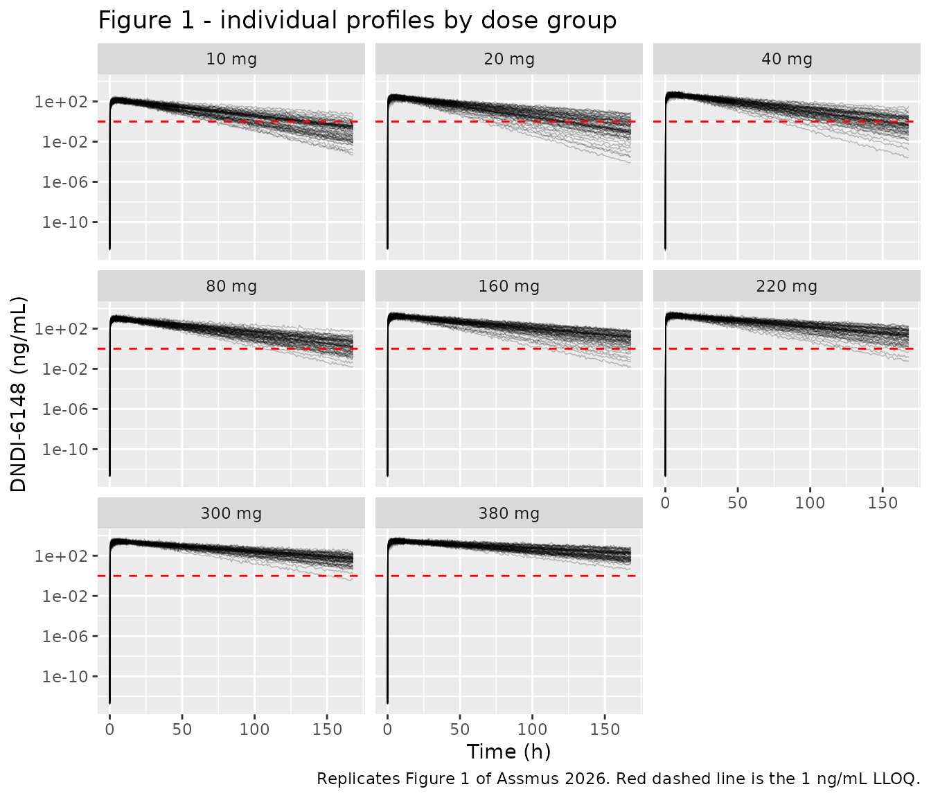

# Bottom-right panel of Figure 1: median concentration by dose group.
sim |>
  dplyr::filter(time <= 168) |>
  dplyr::group_by(cohort, time) |>
  dplyr::summarise(median_ng = median(sim) * 1000, .groups = "drop") |>
  dplyr::filter(median_ng > 0) |>
  ggplot(aes(time, median_ng, colour = cohort)) +
  geom_line(linewidth = 0.7) +
  geom_hline(yintercept = 1, colour = "red", linetype = "dashed") +
  scale_y_log10() +
  labs(x = "Time (h)", y = "Median DNDI-6148 (ng/mL)", colour = "Dose",
       title = "Figure 1, bottom-right panel - median concentration by dose group",
       caption = "Replicates the median overlay panel of Figure 1 of Assmus 2026.")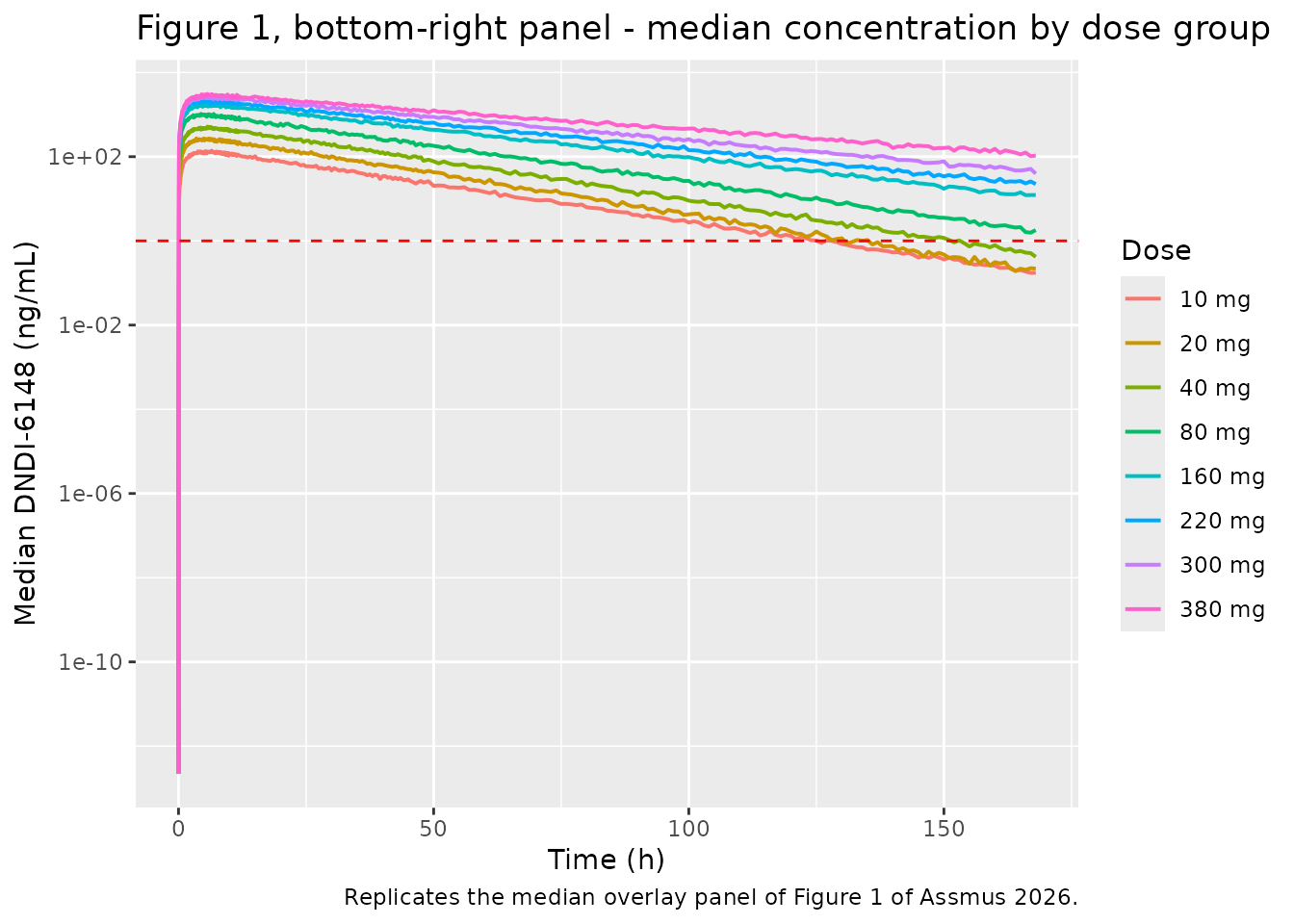

# Replicates S1 Fig: the exponential dose effects used in the final model, with
# the median dose of 1.7 mg/kg marked.
tibble::tibble(mgkg = seq(0.1, 5.6, by = 0.02)) |>
  dplyr::mutate(
    F          = exp(-0.123 * (mgkg - 1.7)),
    `CL/F`     = 2.55 * exp(-0.150 * (mgkg - 1.7))
  ) |>
  tidyr::pivot_longer(c(F, `CL/F`), names_to = "parameter", values_to = "value") |>
  ggplot(aes(mgkg, value)) +
  geom_line(linewidth = 0.8) +
  geom_vline(xintercept = 1.7, linetype = "dashed") +
  facet_wrap(~parameter, scales = "free_y") +
  labs(x = "Dose (mg/kg)", y = "Parameter value",
       title = "S1 Fig - exponential dose effects on F and CL/F",
       caption = paste("Replicates S1 Fig of Assmus 2026. Dashed line is the",
                       "median dose of 1.7 mg/kg, where both effects equal 1."))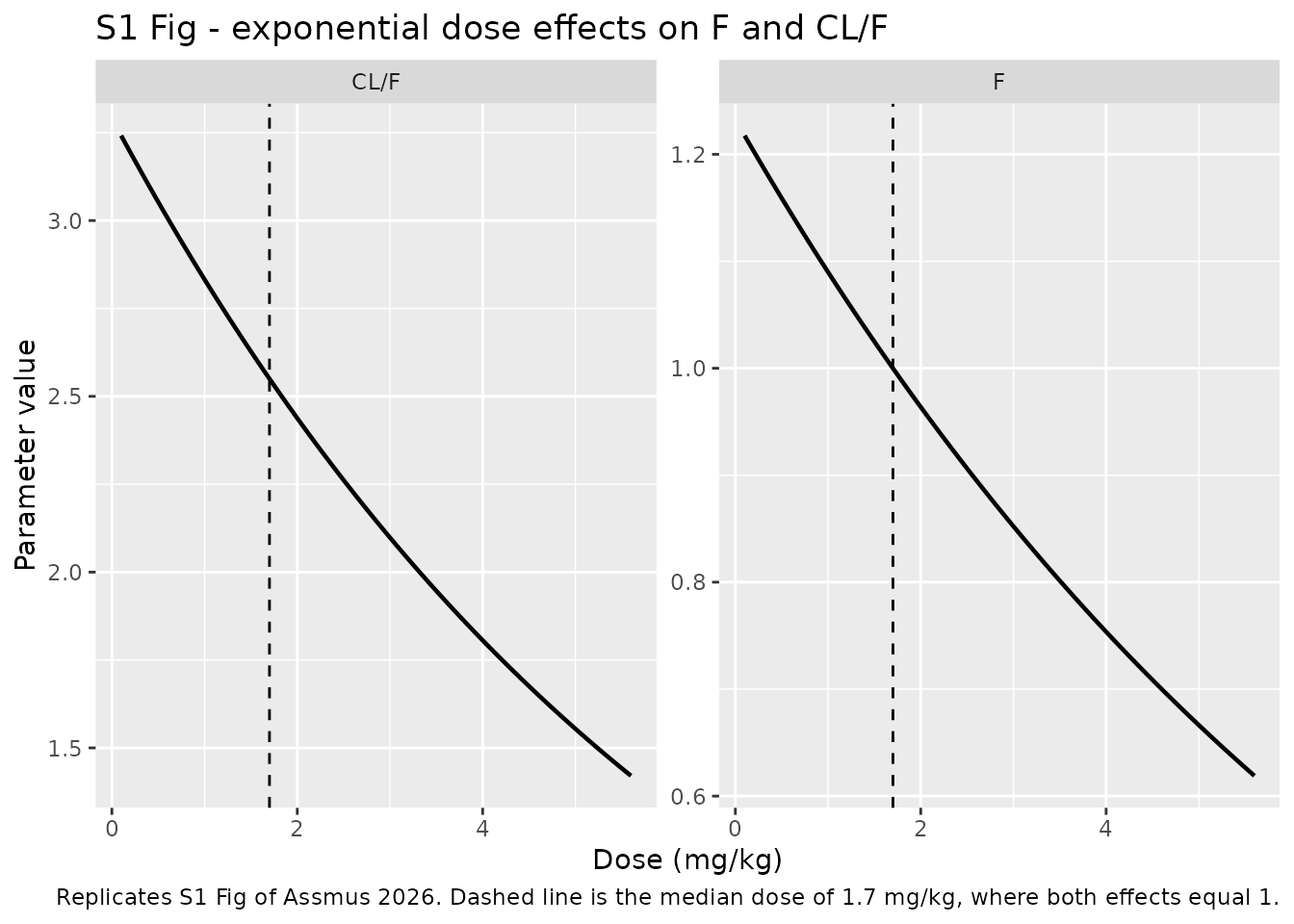

PKNCA validation

Table 3 reports secondary PK parameters derived from the population PK model, so the NCA runs on Cc (the individual prediction) rather than on sim.

sim_nca <- sim |>
  dplyr::filter(!is.na(Cc)) |>
  dplyr::select(id, time, Cc, cohort)

# Guarantee a time = 0 row per (id, cohort); for extravascular dosing a
# pre-dose concentration of zero is the correct anchor for AUC0-*.
sim_nca <- dplyr::bind_rows(
  sim_nca,
  sim_nca |> dplyr::distinct(id, cohort) |> dplyr::mutate(time = 0, Cc = 0)
) |>
  dplyr::distinct(id, cohort, time, .keep_all = TRUE) |>
  dplyr::arrange(id, cohort, time)

stopifnot(nrow(sim_nca) > 0, !anyNA(sim_nca$Cc))

conc_obj <- PKNCA::PKNCAconc(as.data.frame(sim_nca), Cc ~ time | cohort + id)

dose_df <- events |>
  dplyr::filter(evid == 1) |>
  dplyr::select(id, time, amt, cohort) |>
  as.data.frame()

dose_obj <- PKNCA::PKNCAdose(dose_df, amt ~ time | cohort + id)

intervals <- data.frame(
  start      = 0,
  end        = Inf,
  cmax       = TRUE,
  tmax       = TRUE,
  aucinf.obs = TRUE,
  half.life  = TRUE
)

nca_res <- PKNCA::pk.nca(PKNCA::PKNCAdata(conc_obj, dose_obj, intervals = intervals))

nca_wide <- as.data.frame(nca_res) |>
  dplyr::filter(PPTESTCD %in% c("cmax", "tmax", "aucinf.obs", "half.life")) |>
  dplyr::select(cohort, id, PPTESTCD, PPORRES) |>
  tidyr::pivot_wider(names_from = PPTESTCD, values_from = PPORRES)

stopifnot(nrow(nca_wide) == 8L * n_per_arm, !anyNA(nca_wide$aucinf.obs))

Comparison against published NCA

Table 3 gives medians (5th-95th percentile) per dose group. Cmax is printed in ng/mL there and is converted to the model’s ug/mL below so the whole table sits in one unit system; AUCinf is already in ug*h/mL.

published <- tibble::tibble(
  cohort      = dose_labels,
  cmax        = c(138, 265, 590, 1007, 1792, 2184, 2459, 3088) / 1000,  # ng/mL -> ug/mL
  tmax        = c(4.23, 5.23, 5.54, 5.34, 6.13, 5.69, 3.50, 5.91),
  aucinf.obs  = c(3.05, 7.15, 21.4, 34.4, 61.7, 86.9, 113, 159),
  half.life   = c(12.6, 13.2, 20.7, 19.8, 19.9, 22.5, 26.6, 33.7)
)

cmp <- nlmixr2lib::ncaComparisonTable(
  simulated = nca_res,
  reference = published,
  by        = "cohort",
  units     = c(cmax = "ug/mL", aucinf.obs = "ug*h/mL",
                tmax = "h", half.life = "h"),
  tolerance_pct = 20
)

knitr::kable(
  cmp,
  caption = paste("Simulated vs published NCA (Table 3 of Assmus 2026).",
                  "* differs from the reference by more than 20%."),
  align = c("l", "l", "r", "r", "r")
)

Simulated vs published NCA (Table 3 of Assmus 2026). * differs from the reference by more than 20%.
NCA parameter	cohort	Reference	Simulated	% diff
Cmax (ug/mL)	10 mg	0.138	0.134	-3.2%
Cmax (ug/mL)	20 mg	0.265	0.266	+0.2%
Cmax (ug/mL)	40 mg	0.59	0.49	-17.0%
Cmax (ug/mL)	80 mg	1.01	0.987	-1.9%
Cmax (ug/mL)	160 mg	1.79	1.75	-2.4%
Cmax (ug/mL)	220 mg	2.18	2.12	-2.8%
Cmax (ug/mL)	300 mg	2.46	2.57	+4.5%
Cmax (ug/mL)	380 mg	3.09	2.94	-4.8%
Tmax (h)	10 mg	4.23	5	+18.2%
Tmax (h)	20 mg	5.23	4.9	-6.3%
Tmax (h)	40 mg	5.54	5.4	-2.5%
Tmax (h)	80 mg	5.34	4.6	-13.9%
Tmax (h)	160 mg	6.13	4.9	-20.1%*
Tmax (h)	220 mg	5.69	4.95	-13.0%
Tmax (h)	300 mg	3.5	6.2	+77.1%*
Tmax (h)	380 mg	5.91	5.7	-3.6%
AUC0-∞ (obs) (ug*h/mL)	10 mg	3.05	4.17	+36.7%*
AUC0-∞ (obs) (ug*h/mL)	20 mg	7.15	7.87	+10.1%
AUC0-∞ (obs) (ug*h/mL)	40 mg	21.4	15.1	-29.3%*
AUC0-∞ (obs) (ug*h/mL)	80 mg	34.4	31.3	-9.1%
AUC0-∞ (obs) (ug*h/mL)	160 mg	61.7	64	+3.8%
AUC0-∞ (obs) (ug*h/mL)	220 mg	86.9	89.4	+2.9%
AUC0-∞ (obs) (ug*h/mL)	300 mg	113	116	+2.3%
AUC0-∞ (obs) (ug*h/mL)	380 mg	159	163	+2.3%
t½ (h)	10 mg	12.6	17	+34.6%*
t½ (h)	20 mg	13.2	15.9	+20.1%*
t½ (h)	40 mg	20.7	16.1	-22.0%*
t½ (h)	80 mg	19.8	17.8	-9.9%
t½ (h)	160 mg	19.9	22.7	+14.0%
t½ (h)	220 mg	22.5	24.6	+9.5%
t½ (h)	300 mg	26.6	27.5	+3.5%
t½ (h)	380 mg	33.7	36.6	+8.6%

# Per-cohort percentage differences, recomputed so they can be asserted on.
nca_med <- nca_wide |>
  dplyr::group_by(cohort) |>
  dplyr::summarise(dplyr::across(c(cmax, tmax, aucinf.obs, half.life), median),
                   .groups = "drop")

pct <- nca_med |>
  dplyr::inner_join(published, by = "cohort", suffix = c("_sim", "_ref")) |>
  dplyr::mutate(
    cmax       = 100 * (cmax_sim       - cmax_ref)       / cmax_ref,
    tmax       = 100 * (tmax_sim       - tmax_ref)       / tmax_ref,
    aucinf.obs = 100 * (aucinf.obs_sim - aucinf.obs_ref) / aucinf.obs_ref,
    half.life  = 100 * (half.life_sim  - half.life_ref)  / half.life_ref
  ) |>
  dplyr::select(cohort, cmax, tmax, aucinf.obs, half.life)

knitr::kable(pct, digits = 1,
             caption = "Percentage difference from Table 3, per dose cohort and parameter.")

Percentage difference from Table 3, per dose cohort and parameter.
cohort	cmax	tmax	aucinf.obs	half.life
10 mg	-3.2	18.2	36.7	34.6
20 mg	0.2	-6.3	10.1	20.1
40 mg	-17.0	-2.5	-29.3	-22.0
80 mg	-1.9	-13.9	-9.1	-9.9
160 mg	-2.4	-20.1	3.8	14.0
220 mg	-2.8	-13.0	2.9	9.5
300 mg	4.5	77.1	2.3	3.5
380 mg	-4.8	-3.6	2.3	8.6


# The published values are medians of six post-hoc individual estimates per
# cohort, so per-cohort scatter of this size is expected and is NOT a model
# defect -- the median of six draws with a 31% CV on clearance moves around a
# lot. Assert on the CENTRE across cohorts and on a robust quantile, never on
# the worst cohort: the extreme of a random cohort is not reproducible across
# rxode2 builds or thread counts.
#
# Cmax and AUCinf are the structural checks: a mis-transcribed clearance,
# volume, dose or unit moves the whole distribution by tens of percent.
stopifnot(abs(median(pct$cmax)) < 15)
stopifnot(abs(median(pct$aucinf.obs)) < 20)
stopifnot(quantile(abs(pct$cmax), 0.9) < 35)

# Tmax is driven by ka alone, which is shared across cohorts, so its centre is
# the meaningful statistic; the published per-cohort Tmax medians swing from
# 3.50 to 6.13 h on six subjects each.
stopifnot(abs(median(pct$tmax)) < 30)

# Half-life is log(2) * vc / cl in this model; it must track the published
# dose-dependent increase rather than any single cohort's value.
stopifnot(abs(median(pct$half.life)) < 25)

Non-linearity claims

The paper’s central quantitative claims about non-linearity are checked here against the simulated cohort, with bounds wide enough to survive a different draw but narrow enough that a mis-encoded dose effect breaks them.

fold <- nca_med |>
  dplyr::filter(cohort %in% c("10 mg", "380 mg")) |>
  dplyr::arrange(match(cohort, dose_labels))

cmax_fold <- fold$cmax[2] / fold$cmax[1]
auc_fold  <- fold$aucinf.obs[2] / fold$aucinf.obs[1]

tibble::tibble(
  Claim = c(
    "38-fold dose increase gives ~22-fold Cmax increase (Results)",
    "AUCinf increases approximately dose-linearly, i.e. ~38-fold (Results)",
    "Median t1/2 rises from ~13 h (10-20 mg) to ~34 h (380 mg) (Results)"
  ),
  Simulated = c(
    sprintf("%.1f-fold", cmax_fold),
    sprintf("%.1f-fold", auc_fold),
    sprintf("%.1f h -> %.1f h",
            nca_med$half.life[nca_med$cohort == "10 mg"],
            nca_med$half.life[nca_med$cohort == "380 mg"])
  )
) |>
  knitr::kable(caption = "Published non-linearity claims vs the simulated cohort.")

Published non-linearity claims vs the simulated cohort.
Claim	Simulated
38-fold dose increase gives ~22-fold Cmax increase (Results)	22.0-fold
AUCinf increases approximately dose-linearly, i.e. ~38-fold (Results)	39.0-fold
Median t1/2 rises from ~13 h (10-20 mg) to ~34 h (380 mg) (Results)	17.0 h -> 36.6 h


# Dose ratio is 38. If BOTH dose effects were dropped the model would be linear
# and both folds would sit at 38; if only the F effect were dropped, Cmax would
# also be ~38. The Cmax bound therefore goes red on either mis-encoding while
# admitting cohort-to-cohort noise.
stopifnot(cmax_fold > 15, cmax_fold < 30)
stopifnot(auc_fold  > 30, auc_fold  < 55)

# Half-life must increase with dose, because the CL effect is negative while
# volume is dose-independent. This is a large, structural difference (roughly
# 2.5-fold), not a near-zero effect whose sign could flip on a redraw.
hl_lo <- nca_med$half.life[nca_med$cohort == "10 mg"]
hl_hi <- nca_med$half.life[nca_med$cohort == "380 mg"]
stopifnot(hl_hi / hl_lo > 1.8, hl_hi / hl_lo < 3.5)

# Replicates Figure 4 of Assmus 2026: dose-normalised Cmax and AUCinf by dose
# group. A flat series would mean dose proportionality; Cmax/dose declines while
# AUCinf/dose is approximately flat.
nca_wide |>
  dplyr::left_join(
    tibble::tibble(cohort = dose_labels, dose_mg = dose_levels), by = "cohort"
  ) |>
  dplyr::mutate(
    `Cmax/dose (ug/mL per mg)`      = cmax / dose_mg,
    `AUCinf/dose (ug*h/mL per mg)`  = aucinf.obs / dose_mg,
    cohort = factor(cohort, levels = dose_labels)
  ) |>
  tidyr::pivot_longer(
    c(`Cmax/dose (ug/mL per mg)`, `AUCinf/dose (ug*h/mL per mg)`),
    names_to = "parameter", values_to = "value"
  ) |>
  ggplot(aes(cohort, value)) +
  geom_boxplot(outlier.size = 0.5) +
  facet_wrap(~parameter, scales = "free_y") +
  labs(x = "Dose group", y = "Dose-normalised exposure",
       title = "Figure 4 - dose-normalised exposure by dose group",
       caption = "Replicates Figure 4 of Assmus 2026.") +
  theme(axis.text.x = element_text(angle = 45, hjust = 1))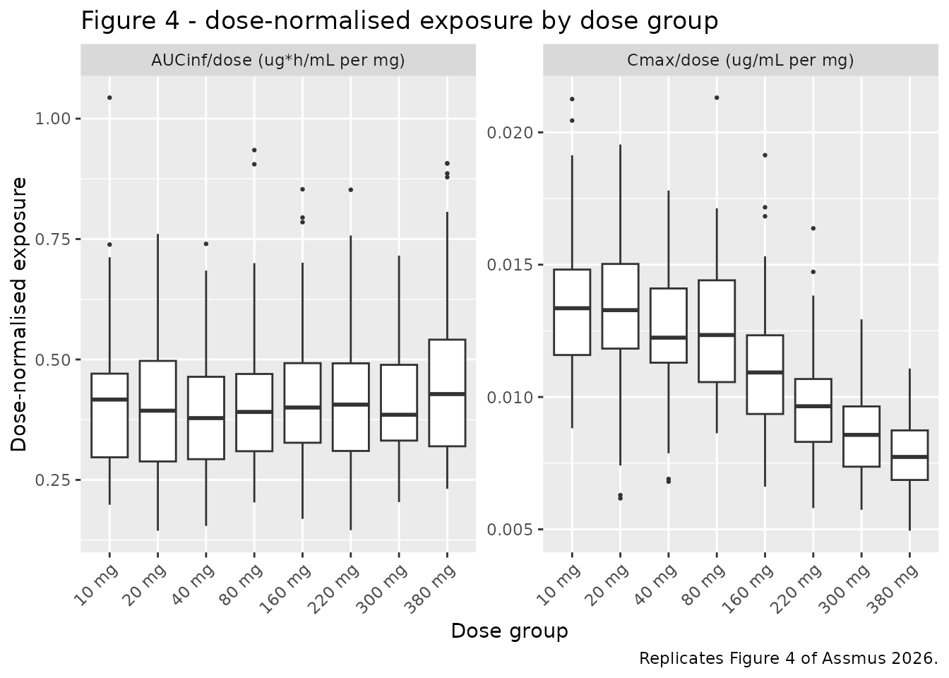

Assumptions and deviations

Body-weight distribution. Table 1 reports only median and range per cohort, not a distribution. A log-normal centred on the pooled median 72.3 kg with a 13% CV, truncated to the observed 56.9-96.5 kg range, is used throughout. The paper’s per-cohort median weights differ (65.3 kg at 20 mg, 84.4 kg at 300 mg) but the pooled distribution is used for every arm, so the simulated mg/kg values differ slightly from Table 1’s per-cohort medians. The V/F gate above sidesteps this by probing the model at Table 1’s own median weights.
IIV on apparent volume is omitted, not written as fixed(0). The S1 Code $OMEGA 2 is 0 FIX and Table 2 reports no IIV row for V/F. Encoding it as etalvc ~ fixed(0) would put a zero on the OMEGA diagonal, making the matrix singular and breaking the Cholesky sampler rxSolve uses. Dropping the eta is numerically identical and the reason is recorded in the model file.
Residual error. The paper reports sigma as a variance on the log-transformed concentration scale (0.0361). This is encoded as Cc ~ lnorm(expSd) with expSd = sqrt(0.0361) = 0.19, the log-scale SD, which is the form nlmixr2 expects. The paper’s own wording – “additive error on log-transformed concentrations, equivalent to an exponential error on the arithmetic scale” – and the S1 Code $ERROR block (IPRED = LOG(CP); Y = IPRED + EPS(1)) both confirm the scale.
A transcription slip in the published S1 Code. The control stream reads CL = TVCL_P * EXP(ETA(1)) and F1 = TVF1 * EXP(ETA(4)), but TVCL_P is never defined – the line immediately above assigns TVCL. The intended TVCL is used here. The stream would not run as printed; nothing about the model structure is ambiguous as a result, and Table 2’s estimates are unaffected.
No LLOQ censoring. The assay LLOQ was 1 ng/mL and the paper states every post-dose sample was above it, so no censoring is applied to the simulated concentrations. Figure 1 marks the LLOQ for reference only.
Emax dose effects not implemented. The authors tested Emax-type saturation models for the dose effects on F and CL/F, which fit marginally better (dOFV = -3.24) but estimated D50 with more than 120% RSE. They retained the exponential form for parsimony, and that is what is packaged here. No Emax parameter values are reported, so the alternative could not be encoded even as a variant.
Covariates screened but not retained. Age, AST, ALT, ALP, total bilirubin, GGT, creatinine clearance and hematocrit were all examined in the stepwise covariate model and none survived backward elimination. They are recorded in the model’s covariatesDataExcluded metadata for provenance and carry no coefficients. Sex and race could not be examined at all: every participant was a White man.
Extrapolation outside 0.12-5.56 mg/kg. Both dose effects are exponential in the difference from 1.7 mg/kg, so they diverge without bound outside the studied range. The authors warn about this explicitly in the Discussion. The simulations here stay inside the studied doses.
Per-cohort NCA scatter. Table 3’s values are medians of six post-hoc individual estimates per dose group. With a 31% CV on clearance and a 56% CV on absorption, the median of six draws is itself noisy, so per-cohort differences of 10-30% between the simulated cohort and Table 3 are expected. The gates above therefore assert on the centre across cohorts and on a robust quantile, never on the worst cohort.