Model and source
- Citation: Zhang H, He Y, Davies Forsman L, Paues J, Werngren J, Niward K, Schon T, Bruchfeld J, Alffenaar J-W, Hu Y (2023). Population pharmacokinetics and dose evaluations of linezolid in the treatment of multidrug-resistant tuberculosis. Frontiers in Pharmacology 13:1032674. doi:10.3389/fphar.2022.1032674. Parameter estimates are from Table 2 (final model, Phoenix NLME 8.0). The covariate equation forms and the reference weight are not printed.
- Description: Two-compartment population PK model for oral linezolid in Chinese adults with multidrug-resistant tuberculosis (Zhang 2022), with first-order absorption after a lag time and linear elimination. Body weight scales CL (exponent 0.75) and the central volume (exponent 1.0) about an assumed 70 kg reference (the paper prints no reference weight); type 2 diabetes adds an additive shift to CL and to the central volume. Residual error is additive. The intercompartmental clearance is encoded as printed (Q = 0.9 L/h); with it the model under-predicts the paper’s own posthoc trough concentrations about twofold, and a value of 9 L/h would reproduce them (see the vignette Errata).
- Article: https://doi.org/10.3389/fphar.2022.1032674 (open access, PMC9868619). The article is in volume 13 (2022) and was published online on 9 January 2023.
Linezolid is a WHO Group A drug for multidrug-resistant tuberculosis (MDR-TB). Zhang et al. developed a population PK model for linezolid 600 mg once daily in Chinese adults with MDR-TB, used it to estimate individual exposures in a separate validation cohort, related AUC0-24/MIC to treatment outcome (threshold 125), and evaluated doses of 300-1400 mg by probability of target attainment (PTA).
Read the Errata section before using this model. It is encoded as printed in Table 2, and with the printed intercompartmental clearance (Q = 0.9 L/h) it predicts trough concentrations about half those the paper itself reports.
Population
The model was developed in 168 participants (1008 plasma samples) of a prospective multicentre cohort in Jiangsu, Guizhou and Sichuan provinces, China, 2015-2017 (Zhang 2022 Methods 2.1; Zheng 2021). Participants were 18 to < 70 years old with laboratory-confirmed MDR-TB; critically ill, pregnant, and HIV-, HBV- or HCV-infected patients were excluded. All received linezolid 600 mg orally once daily with bedaquiline, a fluoroquinolone and a background regimen. Blood was sampled after 2 weeks of inpatient treatment, predose and 1, 2, 4, 6 and 8 h post-dose.
Table 1 (development cohort, median (IQR) or n (%)): age 41 (33-45) years, weight 53 (47-66) kg, BMI 20 (18-23), 125 (74.4%) male, type 2 diabetes 32 (19.0%). The validation cohort (159 participants, Sichuan, Jiangsu and Henan) had weight 59 (53-64) kg, 103 (64.8%) male and type 2 diabetes 27 (17.0%), and was sampled predose, 2 and 6 h post-dose.
The same information is available programmatically via
readModelDb("Zhang_2022_linezolid")()$population.
Source trace
Every value is from Zhang 2022 Table 2. Frontiers typesets decimals
without a leading zero, so the table prints .9,
.6, .75, .1 and
.5.
| Equation / parameter | Value | Source location |
|---|---|---|
lka |
log(2.0 1/h) | Table 2 ‘Ka (/h)’ 2.0, RSD 11.1% |
lcl |
log(5.6 L/h) | Table 2 ‘CL (L/h)’ 5.6, RSD 1.6% |
lvc |
log(35.8 L) | Table 2 ‘V d (L)’ 35.8, RSD 2.0% |
lq |
log(0.9 L/h) | Table 2 ‘Q (L/h)’ .9, RSD 13.7% (see Errata) |
lvp |
log(58.6 L) | Table 2 ‘Vp(L)’ 58.6, RSD 13.2% |
ltlag |
log(0.6 h) | Table 2 ‘Tlag(h)’ .6, RSD 8.4% |
e_wt_cl |
fixed(0.75) | Table 2 ‘theta (Bodyweight)-CL’ .75, no RSD |
e_wt_vc |
fixed(1.0) | Table 2 ‘theta (Bodyweight)-Vd’ 1.0, no RSD |
e_dis_diab_cl |
0.1 L/h | Table 2 ‘theta (Diabetes)-CL’ .1, RSD 10.5% |
e_dis_diab_vc |
5.0 L | Table 2 ‘theta (Diabetes)-Vd’ 5.0, RSD 11.1% |
etalcl |
0.045600 | Table 2 IIV CL 21.6 %CV; log(0.216^2 + 1) |
etalvc |
0.057831 | Table 2 IIV Vd 24.4 %CV; log(0.244^2 + 1) |
addSd |
0.5 mg/L | Table 2 ‘Additional residual (mg/L)’ .5, RSD 4.2% |
| Structure | 2-cmt, first-order absorption with lag, linear elimination | Results 3.3; Methods 2.3; Table 2 |
| Weight model |
(WT/70)^e_wt_cl, (WT/70)^e_wt_vc
|
Form and reference not printed; 70 kg assumed (Assumptions) |
| Diabetes model |
+ e_dis_diab_cl * DIS_DIAB,
+ e_dis_diab_vc * DIS_DIAB
|
Form not printed; additive assumed (Assumptions) |
| Residual error | additive | Results 3.3 ‘An additive error model was used’ |
Virtual cohorts
Two cohorts of 200 participants each, both on linezolid 600 mg once daily for 15 days. The development cohort (Figure 3) draws weight from a log-normal distribution with median 53 kg and the Table 1 IQR 47-66 kg, and 19% have type 2 diabetes. The validation cohort (Table 3, Figure 6) uses median 59 kg (IQR 53-64 kg) and 17% type 2 diabetes. Weights are truncated to 35-100 kg.
set.seed(20230109)
rxode2::rxSetSeed(20230109)

n_per <- 200
dose_days <- 15
obs_times <- sort(unique(c(
  seq(0, 24, by = 0.25),
  seq(336, 360, by = 0.25)
)))

make_cohort <- function(n, wt_median, wt_q1, wt_q3, p_diab, cohort, id_offset = 0L) {
  sdlog <- (log(wt_q3) - log(wt_q1)) / (2 * qnorm(0.75))
  subj <- tibble(
    id = id_offset + seq_len(n),
    WT = pmin(pmax(exp(rnorm(n, log(wt_median), sdlog)), 35), 100),
    DIS_DIAB = rbinom(n, 1, p_diab),
    cohort = cohort
  )
  dose <- subj |>
    tidyr::crossing(time = 24 * (seq_len(dose_days) - 1)) |>
    mutate(evid = 1L, amt = 600, cmt = "depot")
  obs <- subj |>
    tidyr::crossing(time = obs_times) |>
    mutate(evid = 0L, amt = 0, cmt = "central")
  bind_rows(dose, obs) |>
    arrange(id, time, desc(evid))
}

events <- bind_rows(
  make_cohort(n_per, 53, 47, 66, 0.19, "Development", id_offset = 0L),
  make_cohort(n_per, 59, 53, 64, 0.17, "Validation", id_offset = n_per)
)
stopifnot(!anyDuplicated(unique(events[, c("id", "time", "evid")])))

events |>
  distinct(id, cohort, WT, DIS_DIAB) |>
  group_by(cohort) |>
  summarise(
    n = n(),
    `WT median (kg)` = round(median(WT), 1),
    `WT IQR (kg)` = paste(round(quantile(WT, c(0.25, 0.75)), 1), collapse = "-"),
    `Type 2 diabetes (%)` = round(100 * mean(DIS_DIAB), 1),
    .groups = "drop"
  ) |>
knitr::kable(caption = "Simulated cohort covariates.")| cohort | n | WT median (kg) | WT IQR (kg) | Type 2 diabetes (%) |
|---|---|---|---|---|
| Development | 200 | 53.6 | 44.7-63.6 | 19 |
| Validation | 200 | 57.6 | 52.5-64.1 | 16 |
Simulation
mod <- rxode2::rxode(readModelDb("Zhang_2022_linezolid"))
#> ℹ parameter labels from comments will be replaced by 'label()'
sim <- rxode2::rxSolve(
  mod,
  events = events,
  keep = c("cohort", "WT", "DIS_DIAB"),
  returnType = "data.frame"
)
Replicate Figure 3 (steady-state VPC, development cohort)
Figure 3 is a VPC of the development cohort after 2 weeks of treatment. The points overlaid below are the median of the simulated data, read by the maintainers from the centre of the shaded 95% confidence band of Figure 3 (approximately; the figure has no gridlines below 3 mg/L).
fig3_median <- tibble(
  tad = c(1, 2, 4, 6, 8, 24),
  Cc = c(7.4, 7.8, 6.9, 6.1, 5.5, 2.3)
)

vpc <- sim |>
  filter(cohort == "Development", time >= 336) |>
  mutate(tad = time - 336) |>
  group_by(tad) |>
  summarise(
    Q05 = quantile(sim, 0.05),
    Q50 = quantile(sim, 0.50),
    Q95 = quantile(sim, 0.95),
    .groups = "drop"
  )

ggplot(vpc, aes(tad, Q50)) +
  geom_ribbon(aes(ymin = Q05, ymax = Q95), alpha = 0.25, fill = "steelblue") +
  geom_line(colour = "steelblue4") +
  geom_point(data = fig3_median, aes(tad, Cc), colour = "firebrick", size = 2) +
  scale_x_continuous(breaks = seq(0, 24, by = 6)) +
  labs(
    x = "Time after dose (h)", y = "Linezolid concentration (mg/L)",
    title = "Steady state (day 15), development-cohort covariates",
    caption = paste(
      "Line and band: simulated median and 5th-95th percentiles (with residual error).",
      "Points: simulated median read from Zhang 2022 Figure 3.",
      sep = "\n"
    )
  )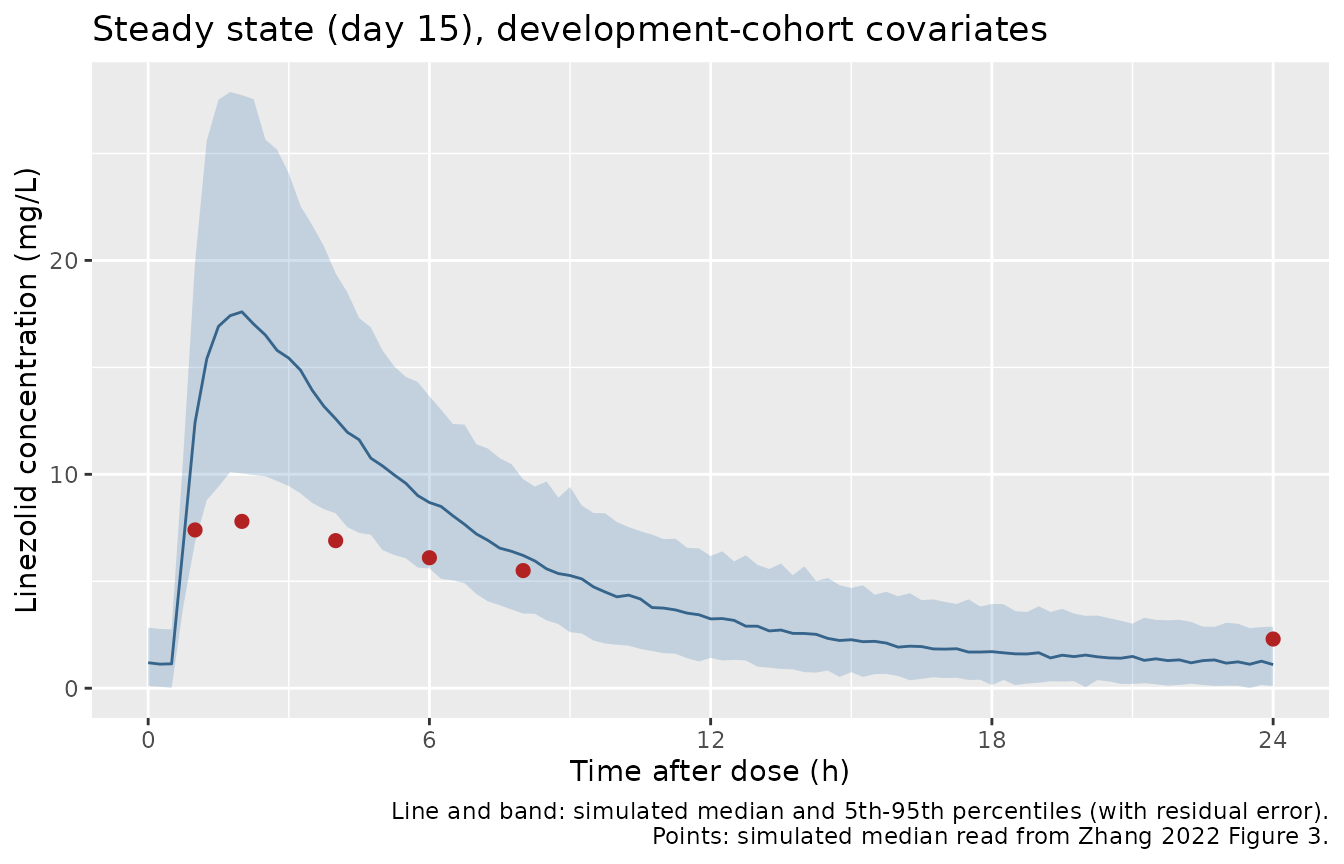
fig3_ratio <- vpc |>
  inner_join(fig3_median, by = "tad") |>
  mutate(ratio = Q50 / Cc)
knitr::kable(
  fig3_ratio |>
    select(tad, Q50, Cc, ratio) |>
    mutate(across(c(Q50, Cc, ratio), ~ round(.x, 2))) |>
    rename(
      "Time after dose (h)" = tad,
      "Simulated median (mg/L)" = Q50,
      "Figure 3 median (mg/L)" = Cc,
      "Ratio" = ratio
    ),
  caption = "Simulated median vs. the Figure 3 simulated median."
)| Time after dose (h) | Simulated median (mg/L) | Figure 3 median (mg/L) | Ratio |
|---|---|---|---|
| 1 | 12.42 | 7.4 | 1.68 |
| 2 | 17.60 | 7.8 | 2.26 |
| 4 | 12.59 | 6.9 | 1.83 |
| 6 | 8.68 | 6.1 | 1.42 |
| 8 | 6.21 | 5.5 | 1.13 |
| 24 | 1.10 | 2.3 | 0.48 |
The packaged model peaks at about 2.3 times the Figure 3 median at 2 h, and its 24 h trough is about 0.5 times the Figure 3 value. The Errata section discusses why.
Steady-state exposure versus Table 3 (PKNCA)
Table 3 reports the individual (Bayesian posthoc) Cmax, Cmin and AUC0-24 of the validation cohort. These are compared with a PKNCA analysis of the day-15 dosing interval (336-360 h) of the simulated validation cohort.
conc_ss <- sim |>
  filter(cohort == "Validation", !is.na(Cc), time >= 336) |>
  mutate(treatment = "600 mg QD") |>
  select(id, time, Cc, treatment)

dose_ss <- events |>
  filter(cohort == "Validation", evid == 1) |>
  mutate(treatment = "600 mg QD") |>
  select(id, time, amt, treatment)

conc_obj <- PKNCA::PKNCAconc(conc_ss, Cc ~ time | treatment + id)
dose_obj <- PKNCA::PKNCAdose(dose_ss, amt ~ time | treatment + id)
intervals <- data.frame(
  start = 336, end = 360,
  cmax = TRUE, cmin = TRUE, auclast = TRUE
)
nca_res <- PKNCA::pk.nca(PKNCA::PKNCAdata(conc_obj, dose_obj, intervals = intervals))
published <- tibble::tribble(
  ~treatment, ~cmax, ~cmin, ~auclast,
  "600 mg QD", 16.2, 2.0, 108.3
)

cmp <- nlmixr2lib::ncaComparisonTable(
  simulated = nca_res,
  reference = published,
  by = "treatment",
  units = c(cmax = "mg/L", cmin = "mg/L", auclast = "mg*h/L"),
  tolerance_pct = 20
)
knitr::kable(
  cmp,
  caption = paste(
    "Simulated (median) vs. Zhang 2022 Table 3 (validation cohort, median).",
    "* differs from the reference by more than 20%."
  )
)| NCA parameter | treatment | Reference | Simulated | % diff |
|---|---|---|---|---|
| Cmax (mg/L) | 600 mg QD | 16.2 | 16.4 | +0.9% |
| Cmin (mg/L) | 600 mg QD | 2 | 1 | -49.9%* |
| AUClast (mg*h/L) | 600 mg QD | 108 | 122 | +12.7% |
Cmax and AUC0-24 agree with Table 3 within about 13%; AUC follows from CL alone (AUC = dose/CL at steady state), so this confirms the clearance and its weight scaling. Cmin is about half the Table 3 value, which is the known deviation described in the Errata.
nca_med <- as.data.frame(nca_res) |>
  filter(PPTESTCD %in% c("cmax", "cmin", "auclast")) |>
  group_by(PPTESTCD) |>
  summarise(median = median(PPORRES), .groups = "drop")
med <- setNames(nca_med$median, nca_med$PPTESTCD)

stopifnot(
  # Structural: a mis-transcribed CL, dose or weight exponent moves the
  # steady-state AUC median by tens of percent. Simulated median is ~+13%.
  abs(100 * (med[["auclast"]] / 108.3 - 1)) < 25,
  abs(100 * (med[["cmax"]] / 16.2 - 1)) < 25,
  # Known deviation, pinned so it cannot change silently: with the printed
  # Q = 0.9 L/h the median trough is ~1.0 mg/L against the paper's 2.0 mg/L.
  med[["cmin"]] > 0.6, med[["cmin"]] < 1.4
)
Readings of Q and the reference weight
Table 2 prints Q as .9 L/h and does not state the
reference weight. The table below re-runs the validation cohort under
four readings: Q of 0.9 L/h (as printed) or 9 L/h, and a reference
weight of 70 kg (as packaged) or the development-cohort median of 53 kg.
Because both weight exponents act on WT / 70, the 53 kg
reading is reproduced exactly by passing WT * 70 / 53; the
diabetes shifts are additive and are unaffected.
Figure 6 PTA values are from the Results text (section 3.6) and, under linear PK, convert to probabilities that the 600 mg AUC0-24 exceeds a threshold: 1400 mg reaching AUC/MIC 125 at MIC 1 mg/L in 93.1% means P(AUC600 >= 53.6) = 93.1%, and 300 mg at MIC 0.25 mg/L (74.2%) and 1200 mg at MIC 1 mg/L (68.6%) both mean P(AUC600 >= 62.5). The probabilities are computed for both the day-1 and the day-15 AUC0-24.
auc_trap <- function(time, conc) sum(diff(time) * (head(conc, -1) + tail(conc, -1)) / 2)

val_events <- events |> filter(cohort == "Validation")
readings <- tidyr::crossing(q = c(0.9, 9), ref_wt = c(70, 53))

reading_summary <- function(q, ref_wt) {
  ev <- val_events |> mutate(WT = WT * 70 / ref_wt)
  s <- rxode2::rxSolve(mod, events = ev, params = c(lq = log(q)), returnType = "data.frame")
  per_id <- s |>
    group_by(id) |>
    summarise(
      auc_d1 = auc_trap(time[time <= 24], Cc[time <= 24]),
      auc_ss = auc_trap(time[time >= 336], Cc[time >= 336]),
      cmax_ss = max(Cc[time >= 336]),
      cmin_ss = Cc[time == 360],
      .groups = "drop"
    )
  tibble(
    q = q, ref_wt = ref_wt,
    cmax_ss = median(per_id$cmax_ss),
    cmin_ss = median(per_id$cmin_ss),
    auc_ss = median(per_id$auc_ss),
    auc_d1 = median(per_id$auc_d1),
    p536_d1 = 100 * mean(per_id$auc_d1 >= 53.6),
    p625_d1 = 100 * mean(per_id$auc_d1 >= 62.5),
    p536_ss = 100 * mean(per_id$auc_ss >= 53.6),
    p625_ss = 100 * mean(per_id$auc_ss >= 62.5)
  )
}

reading_tab <- bind_rows(Map(reading_summary, readings$q, readings$ref_wt))

bind_rows(
  reading_tab |>
    mutate(Reading = paste0("Q ", q, " L/h, ", ref_wt, " kg reference",
                            ifelse(q == 0.9 & ref_wt == 70, " (packaged)", ""))),
  tibble(Reading = "Zhang 2022 (Table 3; Results 3.6)",
         cmax_ss = 16.2, cmin_ss = 2.0, auc_ss = 108.3,
         p536_d1 = 93.1, p625_d1 = 74.2)
) |>
  select(Reading, cmax_ss, cmin_ss, auc_ss, auc_d1, p536_d1, p625_d1, p536_ss, p625_ss) |>
  mutate(across(where(is.numeric), ~ round(.x, 1))) |>
  rename(
    "Cmax ss (mg/L)" = cmax_ss,
    "Cmin ss (mg/L)" = cmin_ss,
    "AUC0-24 ss (mg*h/L)" = auc_ss,
    "AUC0-24 day 1 (mg*h/L)" = auc_d1,
    "P(AUC d1 >= 53.6) %" = p536_d1,
    "P(AUC d1 >= 62.5) %" = p625_d1,
    "P(AUC ss >= 53.6) %" = p536_ss,
    "P(AUC ss >= 62.5) %" = p625_ss
  ) |>
knitr::kable(caption = "Validation-cohort medians and AUC exceedance under four readings (no residual error).")| Reading | Cmax ss (mg/L) | Cmin ss (mg/L) | AUC0-24 ss (mg*h/L) | AUC0-24 day 1 (mg*h/L) | P(AUC d1 >= 53.6) % | P(AUC d1 >= 62.5) % | P(AUC ss >= 53.6) % | P(AUC ss >= 62.5) % |
|---|---|---|---|---|---|---|---|---|
| Q 0.9 L/h, 53 kg reference | 12.9 | 0.9 | 102.1 | 89.0 | 99.0 | 96.0 | 99.0 | 97.5 |
| Q 0.9 L/h, 70 kg reference (packaged) | 16.5 | 1.1 | 124.2 | 105.7 | 100.0 | 100.0 | 100.0 | 100.0 |
| Q 9 L/h, 53 kg reference | 12.2 | 1.8 | 100.0 | 74.1 | 97.5 | 86.0 | 99.5 | 98.0 |
| Q 9 L/h, 70 kg reference | 15.2 | 2.3 | 121.8 | 87.3 | 100.0 | 98.5 | 100.0 | 100.0 |
| Zhang 2022 (Table 3; Results 3.6) | 16.2 | 2.0 | 108.3 | NA | 93.1 | 74.2 | NA | NA |
q9 <- reading_tab |> filter(q == 9, ref_wt == 70)
q09 <- reading_tab |> filter(q == 0.9, ref_wt == 70)
stopifnot(
  # The Q = 9 L/h reading recovers the Table 3 trough (2.0 mg/L) and the
  # printed reading does not; both are medians over 200 subjects.
  abs(q9$cmin_ss / 2.0 - 1) < 0.3,
  q09$cmin_ss / 2.0 < 0.7,
  # Q does not change the steady-state AUC (it is dose/CL for both).
  abs(q9$auc_ss / q09$auc_ss - 1) < 0.05
)
Typical-value profile
typ_events <- rxode2::et(amt = 600, ii = 24, addl = dose_days - 1, cmt = "depot") |>
  rxode2::et(seq(336, 360, by = 0.1), cmt = "central")
typ <- bind_rows(
  lapply(c(53, 70), function(w) {
    rxode2::rxSolve(rxode2::zeroRe(mod), events = typ_events,
                    params = c(WT = w, DIS_DIAB = 0), returnType = "data.frame") |>
      mutate(WT = paste(w, "kg"))
  })
)
#> ℹ omega/sigma items treated as zero: 'etalcl', 'etalvc'
#> ℹ omega/sigma items treated as zero: 'etalcl', 'etalvc'

ggplot(typ, aes(time - 336, Cc, colour = WT)) +
  geom_line() +
  labs(x = "Time after dose on day 15 (h)", y = "Linezolid concentration (mg/L)",
       colour = "Body weight",
       title = "Typical steady-state profile, no type 2 diabetes")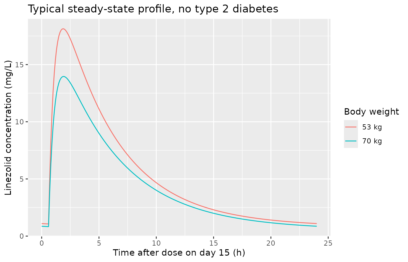
Assumptions and deviations
- Reference weight (assumed 70 kg). Table 2 gives fixed allometric exponents (0.75 on CL, 1.0 on Vd) but no reference weight and no covariate equation. The maintainers used the standard 70 kg. The development-cohort median of 53 kg is the other candidate. With a 53 kg reference, typical CL for a given weight would be 23% higher and the typical volume 32% higher; the “Readings” table above shows both.
- Diabetes effect form (assumed additive). Table 2 gives theta(Diabetes) of 0.1 on CL and 5.0 on Vd without the equation. Read as an exponential (exp(5) = 148-fold), multiplicative (5-fold) or fractional (1 + 5 = 6-fold) effect, 5.0 is implausible for a volume, so both coefficients are encoded as additive shifts in the parameter’s units (CL + 0.1 L/h, Vc + 5.0 L). The additive CL shift is about 2% of the typical CL.
- IIV. Table 2 reports IIV as %CV; it is converted to log-normal variance as omega^2 = log(CV^2 + 1). The CL row is labelled ‘(L/h)’ but sits under ‘Variation of parameters between individuals’ with the Vd row labelled ‘%CV’, so it is read as %CV. No IIV on Ka, Q, Vp or Tlag is reported.
- Bioavailability. Only oral data were modelled; Table 2 labels CL and Vd without ‘/F’. The parameters are apparent (oral) values, and no bioavailability term is included.
- Cohorts. Weight is log-normal with the Table 1 median and IQR, and type 2 diabetes is independent of weight. Age, sex and BMI are not in the model.
Errata
The model is encoded exactly as printed in Table 2. Several of the paper’s own results cannot be reproduced from those values:
-
Trough concentration. Table 3 reports a posthoc
median Cmin of 2.0 mg/L (IQR 1.5-2.3) in the validation cohort. The
packaged model gives about 1.0 mg/L. The Figure 2 goodness-of-fit plots
also place population-predicted troughs at roughly 1.3-2.3 mg/L. A Q of
9 L/h, rather than the printed
.9, recovers the Table 3 trough (see “Readings”) without changing CL or the steady-state AUC. Frontiers typesets decimals without a leading zero, so a lost digit would look like this, but the paper does not correct it and the maintainers have kept the printed value. - Figure 3 VPC. The simulated median in Figure 3 peaks at about 7.8 mg/L and falls almost mono-exponentially to about 2.3 mg/L at 24 h. Neither Q reading reproduces this: a 35.8 L central volume with Ka = 2.0 /h after 600 mg gives a typical peak of 10-18 mg/L, consistent with the Table 3 Cmax of 16.2 mg/L but not with the VPC.
- Figure 6 PTA. Under linear PK the Results-text PTA values imply that only 26-31% of the simulated population had a 600 mg AUC0-24 below 62.5 mg*h/L, i.e. a median AUC0-24 well below the Table 3 steady-state median of 108.3. No steady-state reading reproduces this; a day-1 AUC0-24 with Q = 9 L/h and a 53 kg reference comes closest. The paper does not state which AUC was used in the PTA simulation.
- Steady-state AUC and Cmax reproduce within about 13% of Table 3 with the packaged model, so CL, its weight scaling and the central volume are consistent with the paper.
No correction notice for this article was found on the journal page or in Europe PMC as of 2026-10-16.