Elranatamab (Poels 2025)
Source:vignettes/articles/Poels_2025_elranatamab.Rmd
Poels_2025_elranatamab.Rmd- Citation: Poels KE, Elmeliegy M, Hibma J, Wang D, Musante CJ, Shtylla B. Leveraging quantitative systems pharmacology modeling for elranatamab regimen optimization in relapsed or refractory multiple myeloma. npj Syst Biol Appl. 2025;11:102. doi:10.1038/s41540-025-00585-z. Structural framework adapted from Betts et al. (2019) AAPS J 21:66 (see modellib(‘Betts_2019_pf_06671008_qsp’)) and the cytokine-release framework of Chen et al. (2019) Clin Transl Sci 12:600-608.
- Description: QSP. Quantitative systems pharmacology model of the BCMA x CD3 bispecific antibody elranatamab in relapsed/refractory multiple myeloma, calibrated to MagnetisMM-1 (NCT03269136) and MagnetisMM-3 (NCT04649359). Three compartments (central, peripheral, bone marrow / site of action) carry mass-action BsAb binding to membrane BCMA, soluble BCMA (drug sink) and T-cell CD3, forming BsAb-CD3-BCMA trimers that drive Simeoni-type myeloma-cell killing with time-dependent resistance, IL-6-like cytokine release with dose-to-dose attenuation, cytokine- and trimer-dependent T-cell retention in marrow, and M-protein / free light chain paraprotein read-outs. Builds on the Betts 2019 CD3-bispecific framework; see modellib(‘Betts_2019_pf_06671008_qsp’).
- Article: https://doi.org/10.1038/s41540-025-00585-z
Poels et al. (2025) develop a quantitative systems pharmacology (QSP)
model of elranatamab, an approved BCMA x CD3 bispecific
antibody (BsAb) for relapsed or refractory multiple myeloma (RRMM), and
use it to justify the 76 mg weekly regimen and the step-down to
every-2-weeks (Q2W) and every-4-weeks (Q4W) dosing in persistent
responders. The model extends the CD3-bispecific framework of Betts et
al. (2019) – already in this library as
modellib("Betts_2019_pf_06671008_qsp") – with soluble BCMA
(sBCMA) as a drug sink, myeloma paraprotein read-outs, and the
cytokine-release framework of Chen et al. (2019).
The shipped model carries all 28 ordinary differential equations of
Supplementary Note 1 with the parameter values of Supplementary Tables 2
and 3. The paper reports no residual-error model and no between-subject
random effects: it is a simulation-only QSP model in which
patient-to-patient heterogeneity is expressed by resampling nine
structural parameters (Supplementary Table 1) and five baseline states
(Supplementary Table 2). propSd is therefore
fixed(0).
Population
| Field | Value |
|---|---|
| species | human |
| n_subjects | 120 virtual patients per virtual population; 10 virtual populations calibrated (1200 virtual patients total), drawn from >4000 plausible patients out of 10000 sampled parametrizations |
| n_studies | 2 |
| disease_state | Relapsed or refractory multiple myeloma (RRMM); triple-class refractory and BCMA-treatment naive |
| dose_range | Subcutaneous 80, 130, 215, 360, 600 and 1000 ug/kg QW (MagnetisMM-1 Part 1); 600 then 1000 ug/kg QW or Q2W (Part 1.1); 44 mg then 76 mg QW (Part 2A); 12/32/76 mg on C1D1/C1D4/C1D8 then 76 mg QW, stepping down to 76 mg Q2W after cycle 6 and 76 mg Q4W after cycle 12 (MagnetisMM-3 Cohort A). Simulated dose-escalation arms 16, 28, 44, 76 and 152 mg QW plus 76 mg Q2W. |
| regions | Multicentre international (MagnetisMM-1 C1071001; MagnetisMM-3 C1071003) |
| notes | Calibration data are summarised in Supplementary Table 4: MagnetisMM-1 (C1071001) Part 1 IV n = 23, Part 1 SC n = 30, Part 1 C-D n = 13, Part 1.1 QW n = 7, Part 1.1 Q2W n = 13, Part 2A n = 15; MagnetisMM-3 (C1071003) Part A n = 120. The paper reports no age, weight, sex or race distribution for the calibration cohorts, so those fields are omitted rather than guessed. Virtual-patient baselines were sampled from distributions fitted to pooled MagnetisMM-1 and MagnetisMM-3 Cohort A baseline data (Supplementary Table 2, Figure 2b); ~70% of the virtual population had baseline sBCMA < 100 ng/mL and ~30% >= 100 ng/mL. |
Calibration used the phase 1 MagnetisMM-1 (C1071001, NCT03269136) and the registrational phase 2 MagnetisMM-3 (C1071003, NCT04649359) studies. The paper reports the per-arm sample sizes and dosing schedules (Supplementary Table 4) but no age, weight, sex or race distributions for the calibration cohorts, so those fields are absent from the model metadata rather than guessed.
Model structure
The three anatomical compartments are the central (circulating) compartment, a peripheral distribution compartment, and the bone marrow, which serves as the tumour site of action. In the marrow the BsAb binds membrane BCMA on myeloma cells and CD3 on T cells; the productive BsAb-CD3-BCMA trimer drives myeloma-cell killing and cytokine release. Soluble BCMA, shed in proportion to tumour burden, binds one arm of the BsAb in both compartments to form non-productive dimers – the drug-sink mechanism the paper identifies as the key determinant of response.
| State | Analyte | Units | Specimen |
|---|---|---|---|
| depot | elranatamab | pmol | administration site |
| central | elranatamab | pM | serum |
| peripheral1 | elranatamab | pM | serum |
| target | soluble BCMA | pM | serum |
| complex | elranatamab-soluble BCMA dimer | pM | serum |
| drug_cd3_central | elranatamab-CD3 dimer | pM | serum |
| tcell_central | CD3+ T cells | cells/uL | whole blood |
| cytokine_central | pro-inflammatory cytokine (IL-6) | pg/mL | serum |
| mprotein | monoclonal M-protein | g/L | serum |
| flc | involved serum free light chain | mg/L | serum |
| bonemarrow | elranatamab | pM | tumor |
| target_bonemarrow | soluble BCMA | pM | tumor |
| drug_bcma_bonemarrow | elranatamab-membrane BCMA dimer | pM | tumor |
| complex_bonemarrow | elranatamab-soluble BCMA dimer | pM | tumor |
| drug_cd3_bonemarrow | elranatamab-CD3 dimer | pM | tumor |
| trimer | elranatamab-CD3-BCMA trimer | pM | tumor |
| cycling_cells | multiple myeloma cells | cells/uL | tumor |
| damaged_cells1 | multiple myeloma cells | cells/uL | tumor |
| damaged_cells2 | multiple myeloma cells | cells/uL | tumor |
| damaged_cells3 | multiple myeloma cells | cells/uL | tumor |
| tcell_bonemarrow | CD3+ T cells | cells/uL | tumor |
| cytokine_bonemarrow | pro-inflammatory cytokine (IL-6) | pg/mL | tumor |
| cytokine_transit1 | pro-inflammatory cytokine (IL-6) | pg/mL | not applicable |
| cytokine_transit2 | pro-inflammatory cytokine (IL-6) | pg/mL | not applicable |
| cytokine_transit3 | pro-inflammatory cytokine (IL-6) | pg/mL | not applicable |
| cytokine_transit4 | pro-inflammatory cytokine (IL-6) | pg/mL | not applicable |
| cytokine_transit5 | pro-inflammatory cytokine (IL-6) | pg/mL | not applicable |
| cauc | cumulative cytokine exposure | pg/mL*h | not applicable |
Dosing convention
depot holds a subcutaneous amount in
pmol, because Supplementary Eq 1 writes the absorption flux as
F * ka * [Ab_sc] / Vc; every other drug state holds a
concentration in pM. Doses are therefore converted from
mg to pmol with the elranatamab molecular weight of 148.5 kDa (ELREXFIO
US prescribing information, Description section), so 76 mg = 511,785
pmol.
Poels_2025_elranatamab_qsp_events() performs that
conversion and, critically, emits the Supplementary Eq 37 reset of the
cumulative-cytokine-exposure state as an evid = 6
(multiply) record at each dose time. That reset is a discrete state
assignment which an rxode2 ODE cannot express, so it must come from the
event table; simulating without it silently removes the dose-to-dose
attenuation of cytokine release.
Poels_2025_elranatamab_qsp_events(
  dose_time = c(0, 72, 168),
  dose_mg = c(12, 32, 76),
  obs_time = c(0, 24, 168)
)
#>   id time          amt evid     cmt
#> 1  1    0 8.080808e+04    1   depot
#> 2  1    0 6.733728e-01    6    cauc
#> 3  1    0           NA    0 central
#> 4  1   24           NA    0 central
#> 5  1   72 2.154882e+05    1   depot
#> 6  1   72 1.265089e+00    6    cauc
#> 7  1  168 5.117845e+05    1   depot
#> 8  1  168 2.093491e+00    6    cauc
#> 9  1  168           NA    0 central
Source trace
Every ini() value carries an in-file comment naming its
source location. The table below is generated by parsing those comments
out of the installed model file, so it cannot drift from the model.
| Parameter | ini() value | Source location |
|---|---|---|
| kon_bcma | fixed(0.0054) | Suppl Table 3 Sect 1.1: kon1, fixed internal nonclinical data |
| koff_bcma | fixed(0.162) | Suppl Table 3 Sect 1.1: koff1, fixed internal nonclinical data |
| kon_cd3 | fixed(0.00198) | Suppl Table 3 Sect 1.1: kon2, fixed internal nonclinical data |
| koff_cd3 | fixed(82.17) | Suppl Table 3 Sect 1.1: koff2, fixed internal nonclinical data |
| kdeg_sbcma | fixed(0.01925) | Suppl Table 3 Sect 1.1: kdeg_sBCMA, fixed internal nonclinical data |
| ktr_sbcma_bm_c | fixed(0.1) | Suppl Table 3 Sect 1.1: ktr_sBCMA_BM_c, assumed equal to ktr_c_BM |
| lktr_ab_c_bm | log(0.1) | Suppl Table 3 Sect 1.1: ktr_c_BM, estimated with clinical data |
| lktr_ab_bm_c | log(0.3) | Suppl Table 3 Sect 1.1: ktr_BM_c, estimated with clinical data |
| lka | fixed(log(6.167e-3)) | Suppl Table 3 Sect 1.1: ka, preliminary popPK |
| lfdepot | fixed(log(0.511)) | Suppl Table 3 Sect 1.1: F, preliminary popPK |
| lvc | fixed(log(4.25)) | Suppl Table 3 Sect 1.1: Vc [V1], preliminary popPK |
| lvp | fixed(log(7.8)) | Suppl Table 3 Sect 1.1: Vp [V2], preliminary popPK |
| lq | fixed(log(0.008416)) | Suppl Table 3 Sect 1.1: Q, preliminary popPK |
| lcl | fixed(log(0.0139583)) | Suppl Table 3 Sect 1.1: CL, preliminary popPK; kel = CL/Vc |
| lktc_c_bm | log(0.2) | Suppl Table 3 Sect 1.2: k_TC_c_BM, estimated with clinical data and literature |
| lktc_bm_c | log(0.3893) | Suppl Table 3 Sect 1.2: k_TC_BM_c, estimated with clinical data and literature |
| kel_tc | fixed(0.1046) | Suppl Table 3 Sect 1.2: kel_T, fixed from literature [1] (Betts 2019) |
| lbeta_prod | log(1) | Suppl Table 3 Sect 1.2: beta_prod, estimated from literature [14] |
| lkdeg_cyt | log(0.5) | Suppl Table 3 Sect 1.2: kdeg_cyt, estimated with clinical data and literature |
| lktr_cyt | log(0.625) | Suppl Table 3 Sect 1.2: ktr_cyt, estimated with clinical data and literature |
| kdeg_mprotein | fixed(0.0021) | Suppl Table 3 Sect 1.3: kdeg_Mp, fixed from literature [12] (Mills 2017) |
| kdeg_flc | fixed(0.1733) | Suppl Table 3 Sect 1.3: kdeg_FLC, fixed from literature [13] (Tosi 2013) |
| vbm | fixed(1.75) | Suppl Table 3 Sect 2.2: V_BM, fixed from literature [11,10] |
| lkg0 | log(3.32e-4) | Suppl Table 3 Sect 2.2: kg0, calibrated with clinical data and literature |
| lkg1 | log(1500) | Suppl Table 3 Sect 2.2: kg1, calibrated with clinical data and literature |
| psi_switch | fixed(20) | Suppl Table 3 Sect 2.2: psi, fixed from literature [9] (Simeoni 2004) |
| lalpha_kill | log(0.02) | Suppl Table 3 Sect 2.2: alpha_kill, calibrated with clinical data |
| lkm_kill | log(4.25e-4) | Suppl Table 3 Sect 2.2: km, estimated with clinical data and literature |
| ln_kill | log(0.8) | Suppl Table 3 Sect 2.2: n_kill, calibrated with clinical data |
| ltau_mm | log(24) | Suppl Table 3 Sect 2.2: tau_M [tau TA], calibrated with clinical data and literature |
| lmm_max | log(3e6) | Suppl Table 3 Sect 2.2: MM_max, estimated with clinical data |
| lalpha_resis | log(0.5) | Suppl Table 3 Sect 2.2: alpha_resis, calibrated with clinical data |
| lbeta_resis | log(0.1) | Suppl Table 3 Sect 2.2: beta_resis, calibrated with clinical data |
| ltau_resis | log(600) | Suppl Table 3 Sect 2.2: tau_resis, estimated with clinical data |
| lbcma_density | log(12590) | Suppl Table 3 Sect 2.2: BCMA density, calibrated with clinical data and literature [3] |
| lcd3_density | log(6e4) | Suppl Table 3 Sect 2.3: CD3 density, calibrated with clinical data and literature [5] |
| cr_imax | fixed(1) | Suppl Table 3 Sect 2.3: Imax, fixed from literature [2] |
| cr_n_ih | fixed(2.5) | Suppl Table 3 Sect 2.3: n1C, fixed from literature [2] |
| cr_ic50 | fixed(10000) | Suppl Table 3 Sect 2.3: IC50, from literature [2] |
| cr_emax | fixed(80590) | Suppl Table 3 Sect 2.3: Emax, from literature [2] |
| cr_ec50 | fixed(0.5) | Suppl Table 3 Sect 2.3: EC50, from literature [2] |
| cr_n | fixed(1) | Suppl Table 3 Sect 2.3: n2C, from literature [2] |
| imax_tc | fixed(1) | Suppl Table 3 Sect 2.3: Imax_TC, estimated (value at the bound) |
| lksat_tc | log(150) | Suppl Table 3 Sect 2.3: K1, estimated |
| lksat_trimer_tc | log(0.02) | Suppl Table 3 Sect 2.3: K2, estimated |
| ln_cytokine_tc | log(2) | Suppl Table 3 Sect 2.3: n_cyt, estimated |
| ln_trimer_tc | log(1.5) | Suppl Table 3 Sect 2.3: n_tri, estimated |
| eps_kill | fixed(1e-6) | Suppl Sect 1.2.2, value not reported |
| lsbcma0_central | log(5329) | Suppl Table 2: sBCMA_c range; default = geometric midpoint, no point estimate published |
| ltcell0_central | log(203) | Suppl Table 2: Tc_c range; default = geometric midpoint, no point estimate published |
| lmm0 | log(2.25e5) | Suppl Table 2: MM range; default = arithmetic midpoint (range starts at 0, so no geometric midpoint exists) |
| lmprotein0 | log(18.7) | Suppl Table 2: M_P range; default = geometric midpoint of 5-70 g/L, 5 g/L being the IMWG measurability floor the paper cites |
| lflc0 | log(400.9) | Suppl Table 2: FLC range; default = geometric midpoint, no point estimate published |
| cytokine0_central | fixed(2.857) | Suppl Table 2: C_c initial value, reported explicitly |
| sbcma_pm_per_ngml | fixed(185) | derived from the paper’s own two scales: Suppl Table 2 range 185-153520 pM equals the 1-830 ng/mL plausible-patient range of Figure 2b |
| propSd | fixed(0) | the source is a simulation-only QSP model and reports no residual-error model |
| Model element | Source location |
|---|---|
| d/dt(central) - free BsAb in circulation | Suppl Note 1 Eq 1 |
| d/dt(target) - free sBCMA in circulation | Suppl Note 1 Eqs 2-3 |
| d/dt(complex) - BsAb-sBCMA dimer, central | Suppl Note 1 Eq 4 |
| d/dt(drug_cd3_central) - BsAb-CD3 dimer, central | Suppl Note 1 Eq 5 |
| d/dt(tcell_central) - circulating T cells | Suppl Note 1 Eq 6 |
| d/dt(cytokine_central) - circulating cytokine | Suppl Note 1 Eq 7 |
| CD3 receptor pool, central | Suppl Note 1 Eqs 8-10 |
| d/dt(mprotein), d/dt(flc) - paraproteins | Suppl Note 1 Eqs 11-12 |
| d/dt(bonemarrow) - free BsAb in bone marrow | Suppl Note 1 Eq 13 |
| d/dt(target_bonemarrow) - free sBCMA in bone marrow | Suppl Note 1 Eq 14 |
| d/dt(drug_bcma_bonemarrow) - BsAb-BCMA dimer | Suppl Note 1 Eq 15 |
| d/dt(complex_bonemarrow) - BsAb-sBCMA dimer, marrow | Suppl Note 1 Eqs 16-17 |
| d/dt(drug_cd3_bonemarrow) - BsAb-CD3 dimer, marrow | Suppl Note 1 Eq 18 |
| d/dt(trimer) - BsAb-CD3-BCMA trimer | Suppl Note 1 Eq 19 |
| BCMA and CD3 receptor pools, marrow | Suppl Note 1 Eqs 20-23 |
| d/dt(cycling_cells), d/dt(damaged_cells1-3) - Simeoni growth and kill | Suppl Note 1 Eqs 24-27 |
| KMkill - trimer-driven kill rate | Suppl Note 1 Sect 1.2.2 (unnumbered) |
| km_kill_t - time-dependent resistance | Suppl Note 1 Sect 1.2.2 (unnumbered) |
| d/dt(tcell_bonemarrow) - marrow T cells | Suppl Note 1 Eq 28 |
| t_inh - T-cell egress inhibition | Suppl Note 1 Eq 29 |
| d/dt(cytokine_bonemarrow), d/dt(cytokine_transit1-5), d/dt(cauc) | Suppl Note 1 Eqs 30-36 |
| cauc reset at each dose (event-table evid = 6) | Suppl Note 1 Eq 37 |
| IH and Rsyn - cytokine release inhibition and rate | Suppl Note 1 Eq 38 |
| trimerFraction - standardised trimer proportion | Suppl Note 1 Eq 39 |
| Initial conditions of every state | Suppl Table 2 |
| sBCMA pM <-> ng/mL scale (185 pM per ng/mL) | Suppl Table 2 range vs Fig 2b axis |
| Elranatamab molecular weight 148.5 kDa | ELREXFIO USPI, Description |
The reference patient
The paper publishes sampling ranges, not point estimates, for the five sampled baseline states: every published result comes from a 120-patient virtual population. The shipped defaults are therefore the geometric midpoint of each published range (Figure 2b shows all of these distributions are strongly right-skewed, which rules out the arithmetic midpoint), and they are not presented as published estimates. They are listed in Assumptions and deviations below.
| Quantity | Default | Published range (Suppl Table 2) |
|---|---|---|
| Free sBCMA, central | 5329 pM (28.8 ng/mL) | 185-153520 pM (1-830 ng/mL) |
| CD3+ T cells, central | 203 cells/uL | 16-2580 cells/uL |
| Myeloma burden, marrow | 225,000 cells/uL | 0-450000 cells/uL |
| Serum M-protein | 18.7 g/L | 0-70 g/L |
| Involved serum FLC | 401 mg/L | 0.92-174680 mg/L |
Structural checks on the untreated system
Supplementary Sections 1.1.1 and 1.2.1 state that the system is at
steady state at t = 0. Three exact identities follow, and
the untreated model must satisfy all three.
untreated <- solve_untreated(seq(0, 3000, by = 10))
first_last <- untreated[c(1L, nrow(untreated)), ]

## (1) T cells are conserved at baseline in both compartments.
tcell_drift <- max(abs(untreated$tcell_central / untreated$tcell_central[1] - 1),
                   abs(untreated$tcell_bonemarrow / untreated$tcell_bonemarrow[1] - 1))

## (2) With no trimer there is no cytokine release, so circulating cytokine
##     relaxes to the basal balance beta_prod / kdeg_cyt.
cyt_ss_expected <- exp(th[["lbeta_prod"]]) / exp(th[["lkdeg_cyt"]])
cyt_ss_observed <- untreated$cytokineSerum[nrow(untreated)]

## (3) Untreated myeloma grows at kg0 while burden is far below MMmax, so the
##     doubling time approaches log(2) / kg0 exactly. Measured on a low-burden
##     patient (1% of the published baseline range) so the logistic term is
##     negligible and this is a true identity rather than an approximation.
doubling_time <- function(sim) {
  late <- sim[sim$time >= 1000, ]
  log(2) / coef(lm(log(late$tumorBurden) ~ late$time))[[2]] / 24
}
dt_expected_days <- log(2) / exp(th[["lkg0"]]) / 24
untreated_low <- solve_untreated(seq(0, 3000, by = 10),
                                 params = c(lmm0 = log(4500)))
dt_low_days <- doubling_time(untreated_low)
dt_ref_days <- doubling_time(untreated)| Check | Model | Expected |
|---|---|---|
| Max relative drift in T cells (both compartments) | 0.00e+00 | 0 (exact conservation) |
| Circulating cytokine at t = 3000 h (pg/mL) | 2.0000 | 2.0000 (= beta_prod / kdeg_cyt) |
| Doubling time, low-burden patient (days) | 87.2 | 87.0 (= log(2) / kg0) |
| Doubling time, reference patient (days) | 100.8 | > 87.0 (logistic term slows growth) |
Note that the baseline circulating cytokine value in Supplementary
Table 2 (2.857 pg/mL) is not the model’s own basal
steady state (beta_prod / kdeg_cyt = 2.00 pg/mL), so an
untreated simulation relaxes from the tabulated initial condition to
2.00 pg/mL within a few hours. Both values are transcribed exactly as
published; the discrepancy is noted below.
Pharmacokinetics
A single 76 mg subcutaneous dose, with the QSP binding and marrow-transport terms active.
pk <- solve_qsp(dose_time = 0, dose_mg = 76, obs_time = seq(0, 2016, by = 6))
pk$conc_ugml <- pm_to_ugml(pk$Cc)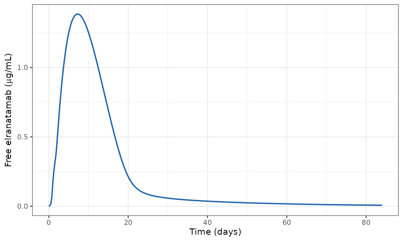
Free elranatamab in serum after a single 76 mg SC dose.
NCA
The model applies bioavailability internally at the depot, so the NCA
dose is the absorbed amount; clearance from
Dose/AUC is then comparable to the model’s CL
rather than to CL/F.
f_sc <- exp(th[["lfdepot"]])
dose_absorbed_mg <- 76 * f_sc

nca_single <- pk |>
  dplyr::transmute(id = id, treatment = "76 mg SC single dose",
                   time = time, Cc = conc_ugml)
dose_single <- data.frame(id = 1L, treatment = "76 mg SC single dose",
                          time = 0, amt = dose_absorbed_mg)

nca_res <- suppressWarnings(as.data.frame(PKNCA::pk.nca(PKNCA::PKNCAdata(
  PKNCA::PKNCAconc(nca_single, Cc ~ time | treatment + id,
                   concu = "ug/mL", timeu = "h"),
  PKNCA::PKNCAdose(dose_single, amt ~ time | treatment + id, doseu = "mg"),
  intervals = data.frame(start = 0, end = Inf, cmax = TRUE, tmax = TRUE,
                         auclast = TRUE, half.life = TRUE)
))))
The label’s clearance is a steady-state value
(“0.324 L/day following 24 weeks dosing”), so the matching simulated
quantity is Dose/AUCtau over the last complete weekly
interval of a 24-week weekly regimen – not a single-dose
AUCinf, which over any tractable observation window would
be dominated by extrapolation.
ss_end <- 24 * 168
ss_dose_t <- c(prime_time, qw_times(336, ss_end))
ss_dose_mg <- c(prime_mg, rep(76, length(ss_dose_t) - 3L))
ss <- solve_qsp(ss_dose_t, ss_dose_mg, seq(0, ss_end, by = 2))
ss$conc_ugml <- pm_to_ugml(ss$Cc)

last_dose_t <- max(ss_dose_t[ss_dose_t <= ss_end - 168])
nca_ss_res <- suppressWarnings(as.data.frame(PKNCA::pk.nca(PKNCA::PKNCAdata(
  PKNCA::PKNCAconc(
    dplyr::transmute(ss, id = id, treatment = "76 mg QW, week 24",
                     time = time, Cc = conc_ugml),
    Cc ~ time | treatment + id, concu = "ug/mL", timeu = "h"),
  PKNCA::PKNCAdose(
    data.frame(id = 1L, treatment = "76 mg QW, week 24",
               time = last_dose_t, amt = dose_absorbed_mg),
    amt ~ time | treatment + id, doseu = "mg"),
  intervals = data.frame(start = last_dose_t, end = last_dose_t + 168,
                         auclast = TRUE, cmax = TRUE, cmin = TRUE)
))))| NCA parameter | Simulated | Reference | Source |
|---|---|---|---|
| Cmax, single dose (ug/mL) | 1.39 | - | - |
| Tmax, single dose (days) | 7.2 | 7 (median, range 3-7) | ELREXFIO USPI 12.3 |
| AUC0-last, single dose (ug*h/mL) | 458 | - | - |
| t1/2 (days) | 18.9 | 22 (64% CV) | ELREXFIO USPI 12.3 |
| Cmax at steady state (ug/mL) | 13.3 | - | - |
| Ctrough at steady state (ug/mL) | 12.4 | - | - |
| AUCtau at steady state (ug*h/mL) | 2193 | - | - |
| CL at steady state (L/day) | 0.425 | 0.324 | ELREXFIO USPI 12.3 |
All three label comparisons are genuine out-of-sample checks: the model’s PK parameters came from the paper’s own preliminary popPK, and no ELREXFIO label value entered the extraction except the molecular weight.
- Tmax is 7.2 days against the label’s median of 7 days. The trial’s PK sampling was on nominal study days, so the label’s “7” is a visit label rather than a resolved maximum.
- Terminal half-life is 18.9 days against the label’s 22 days (64% CV). Note this is shorter than the 47 days the linear two-compartment parameters alone would give, because the QSP layer eliminates the BsAb-sBCMA dimer at the same rate as free drug and so adds a target-mediated component.
-
Steady-state clearance is 0.425 L/day against the
label’s 0.324 L/day, and the paper’s own linear
CL = 0.335L/day sits between them.
The one quantity that does not line up is volume: the label reports a
steady-state volume of 7.76 L against the model’s
Vc + Vp = 12.05 L. The paper’s PK parameters are explicitly
labelled “Preliminary PopPK” – an interim fit available when the QSP
work was done – so a difference from the final label popPK is a property
of the published parameter set, not of the transcription.
MagnetisMM-3 Cohort A regimen
The registrational regimen is 12 mg on C1D1, 32 mg on C1D4 and 76 mg on C1D8, weekly thereafter (Supplementary Table 4).
mm3_end <- 6 * CYCLE_H
mm3_dose_t <- c(prime_time, qw_times(336, mm3_end))
mm3_dose_mg <- c(prime_mg, rep(76, length(mm3_dose_t) - 3L))
mm3 <- solve_qsp(mm3_dose_t, mm3_dose_mg, seq(0, mm3_end, by = 6))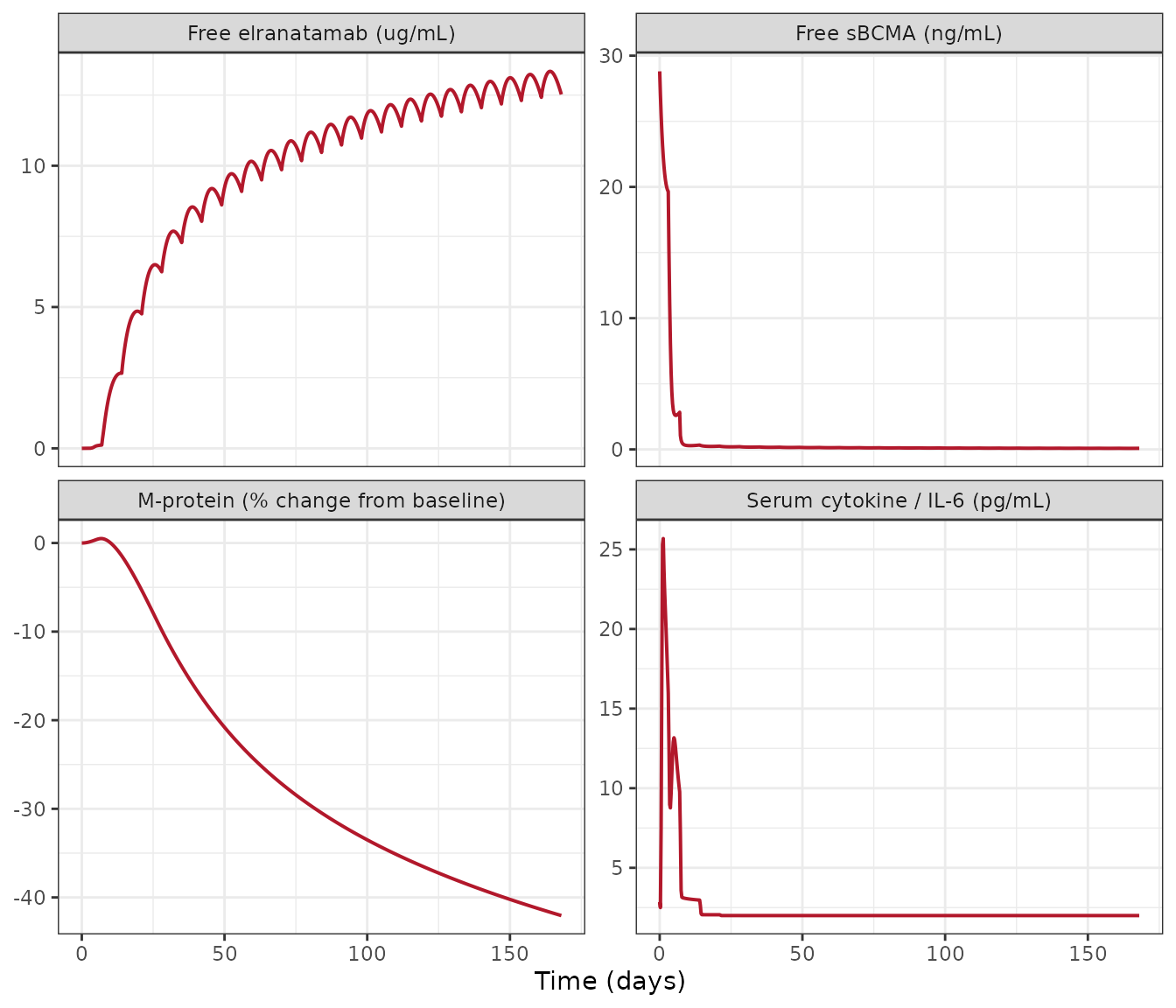
Reference-patient dynamics under the MagnetisMM-3 Cohort A regimen. Replicates the shape of Figure 2c (paraprotein), Supplementary Figure 7 (free sBCMA) and Supplementary Figure 8 (IL-6).
Cytokine-release attenuation (Supplementary Figure 8)
Supplementary Figure 8 shows IL-6 peaking during the priming doses
and then returning to baseline as repeated dosing inflates the
cumulative-exposure state and drives the inhibition term IH
toward Imax. The model reproduces that attenuation, which
is what the Supplementary Eq 37 reset exists to produce.
peak_after <- function(sim, t0) max(sim$cytokineSerum[sim$time >= t0 & sim$time <= t0 + 160])
cyt_peaks <- vapply(mm3_dose_t[1:8], function(t0) peak_after(mm3, t0), numeric(1))

## Same regimen with the Eq 37 reset suppressed.
mm3_noreset <- solve_qsp(mm3_dose_t, mm3_dose_mg, seq(0, mm3_end, by = 6),
                         cytokine_reset = FALSE)
cyt_peaks_noreset <- vapply(mm3_dose_t[1:8], function(t0) peak_after(mm3_noreset, t0), numeric(1))| Dose | Day | Peak cytokine, with Eq 37 reset (pg/mL) | Peak cytokine, reset suppressed (pg/mL) |
|---|---|---|---|
| 1 | 0 | 25.68 | 25.68 |
| 2 | 3 | 15.97 | 16.95 |
| 3 | 7 | 9.77 | 10.28 |
| 4 | 14 | 2.97 | 5.42 |
| 5 | 21 | 2.05 | 4.26 |
| 6 | 28 | 2.00 | 3.73 |
| 7 | 35 | 2.00 | 3.43 |
| 8 | 42 | 2.00 | 3.22 |
Peak cytokine falls from 25.7 pg/mL after the 12 mg priming dose to 3.0 pg/mL by the fourth dose and is back at the basal balance by the sixth. Suppressing the Eq 37 reset raises the fourth-dose peak to 5.4 pg/mL, confirming the reset is load-bearing rather than cosmetic.
Bell-shaped dose-response (Figure 4)
The paper’s central mechanistic claim is that trimer formation – and hence efficacy – is not monotone in dose: at high concentrations the BsAb saturates BCMA and CD3 separately, producing an excess of non-productive dimers at the expense of trimers. Figure 4 plots the “effective binding ratio” (trimers per BCMA receptor) against average drug concentration for the five simulated weekly doses; Supplementary Figure 10 classifies each virtual patient as increasing, bell-shaped or decreasing.
sim_doses <- c(16, 28, 44, 76, 152)
bell_end <- 3 * CYCLE_H

binding_curve <- function(params = NULL) {
  purrr_rows <- lapply(sim_doses, function(d) {
    dt <- qw_times(0, bell_end)
    s <- solve_qsp(dt, rep(d, length(dt)), seq(0, bell_end, by = 6), params = params)
    data.frame(dose_mg = d, conc = mean(s$Cc), binding_ratio = mean(s$bindingRatio))
  })
  do.call(rbind, purrr_rows)
}

curves <- dplyr::bind_rows(
  cbind(phenotype = "Reference patient", binding_curve()),
  cbind(phenotype = "High T cells (2000/uL)",
        binding_curve(c(ltcell0_central = log(2000)))),
  cbind(phenotype = "Low T cells (30/uL)",
        binding_curve(c(ltcell0_central = log(30))))
)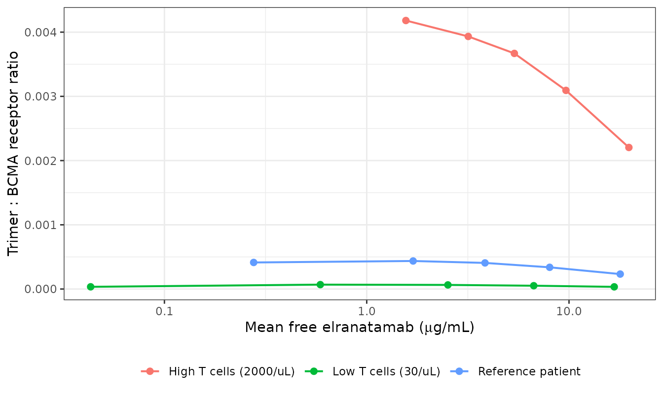
Effective binding ratio (trimers per BCMA receptor) versus mean drug concentration over the first three cycles, for three T-cell phenotypes. Replicates Figure 4a.
| phenotype | Peak dose (mg QW) | Curve shape |
|---|---|---|
| High T cells (2000/uL) | 16 | decreasing |
| Low T cells (30/uL) | 28 | bell-shaped |
| Reference patient | 28 | bell-shaped |
The reference patient peaks at 28 mg weekly and loses 47% of its peak binding ratio at 152 mg – the bell shape of Figure 4a. The three published curve types of Supplementary Figure 10 are recovered by varying baseline T-cell count alone, matching the paper’s finding that marrow T-cell concentration is one of the two most predictive features of curve shape.
Baseline sBCMA as a drug sink
The paper identifies 100 ng/mL as the baseline sBCMA threshold that best separates biochemical responders from non-responders (by iterative logistic regression; Methods), and calibrates two distinct dose-response curves either side of it (Figure 2a). Sweeping the reference patient’s baseline sBCMA across the whole published range reproduces a sharp efficacy cliff.
sbcma_levels_ngml <- c(1, 10, 30, 60, 100, 150, 200, 400, 830)
sbcma_sweep <- lapply(sbcma_levels_ngml, function(ng) {
  s <- solve_qsp(mm3_dose_t, mm3_dose_mg, seq(0, mm3_end, by = 24),
                 params = c(lsbcma0_central = log(ng * PM_PER_NGML)))
  data.frame(
    sbcma_ngml = ng,
    mean_trimer = mean(s$trimer),
    best_pcfb = 100 * (min(s$mProtein) / s$mProtein[1] - 1)
  )
}) |>
dplyr::bind_rows()| Baseline sBCMA (ng/mL) | Mean trimer (pM) | Best M-protein change from baseline (%) | Biochemical response |
|---|---|---|---|
| 1 | 0.8140 | -41.1 | no |
| 10 | 0.8220 | -39.3 | no |
| 30 | 0.8580 | -42.2 | no |
| 60 | 0.9160 | -49.3 | no |
| 100 | 1.0400 | -55.9 | yes |
| 150 | 0.2290 | 0.0 | no |
| 200 | 0.0906 | 0.0 | no |
| 400 | 0.0168 | 0.0 | no |
| 830 | 0.0035 | 0.0 | no |
For this patient the response is lost between 100 and 150 ng/mL – bracketing the 100 ng/mL cut-off the authors derived independently from the clinical data – and mean trimer collapses by a factor of 297 across the full sBCMA range.
Note the small non-monotonicity below the cliff: response improves slightly from 1 to 100 ng/mL. That is the bell shape of the previous section, not a transcription error – a modest sBCMA sink lowers free drug and moves a patient who is past the trimer peak back toward it. The drug-sink effect dominates only once sBCMA is large enough to strip trimer formation outright.
Virtual population
The paper builds each virtual population in two steps: sample 10,000 parametrizations, filter to plausible patients on untreated tumour doubling time, then use a genetic algorithm to select 120 virtual patients whose summary statistics match the observed biochemical response rates and paraprotein trajectories. The second step cannot be reproduced here: its objective-function targets (the per-arm observed BRRs and median trajectories) appear only in figures, and the plausibility bounds on doubling time are not published. What follows is therefore the plausible population, sampled exactly as Supplementary Table 1 describes, and its absolute response rates are expected to sit below the published ones.
n_vp <- 120   # the paper's virtual-population size

runif_fold <- function(n, v, fold) stats::runif(n, v / fold, v * fold)
runif_pct <- function(n, v, pct) stats::runif(n, v * (1 - pct), v * (1 + pct))
runif_log <- function(n, lo, hi) stats::runif(n, log(lo), log(hi))

vp_params <- data.frame(
  id = seq_len(n_vp),
  ## Nine perturbed structural parameters, Supplementary Table 1.
  ## Sampled uniformly on the linear scale, as the paper states.
  lcd3_density  = log(runif_pct(n_vp, 6e4, 0.25)),
  lbcma_density = log(runif_pct(n_vp, 1.259e4, 0.25)),
  lbeta_resis   = log(runif_fold(n_vp, 0.1, 2)),
  lalpha_resis  = log(runif_fold(n_vp, 0.5, 2)),
  lkg0          = log(runif_fold(n_vp, 3.32e-4, 10)),
  lkg1          = log(runif_fold(n_vp, 1500, 10)),
  lalpha_kill   = log(runif_fold(n_vp, 0.02, 10)),
  ltau_mm       = log(stats::runif(n_vp, 24, 30)),
  ln_kill       = log(stats::runif(n_vp, 0.5, 1.5)),
  ## Five sampled baseline states, Supplementary Table 2, drawn LOG-uniformly
  ## over the published ranges (see Assumptions and deviations).
  lsbcma0_central = runif_log(n_vp, 185, 153520),
  ltcell0_central = runif_log(n_vp, 16, 2580),
  lmm0            = runif_log(n_vp, 450, 450000),
  lmprotein0      = runif_log(n_vp, 5, 70),
  lflc0           = runif_log(n_vp, 0.92, 174680)
)

vp <- solve_qsp(mm3_dose_t, mm3_dose_mg, seq(0, mm3_end, by = 24),
                params = vp_params, n_id = n_vp)
#> Warning: multi-subject simulation without without 'omega'

## Biochemical response, per the paper's definition: a >= 50% decrease from
## baseline in the integrated paraprotein, sustained over two consecutive
## (3-weekly) tumour assessments.
assess_h <- seq(0, mm3_end, by = 21 * 24)
vp_resp <- vp |>
  dplyr::filter(time %in% assess_h) |>
  dplyr::group_by(id) |>
  dplyr::arrange(time, .by_group = TRUE) |>
  dplyr::summarise(
    baseline_sbcma = dplyr::first(sbcmaFree),
    baseline_mp = dplyr::first(mProtein),
    pcfb_best = 100 * (min(mProtein) / dplyr::first(mProtein) - 1),
    responder = {
      hit <- mProtein / dplyr::first(mProtein) <= 0.5
      any(hit & dplyr::lead(hit, default = FALSE))
    },
    .groups = "drop"
  ) |>
  dplyr::mutate(sbcma_group = ifelse(baseline_sbcma >= 100,
"high (>= 100 ng/mL)", "low (< 100 ng/mL)"))| Baseline sBCMA | Virtual patients | Share of population (%) | Biochemical response rate (%) | Median best change from baseline (%) |
|---|---|---|---|---|
| high (>= 100 ng/mL) | 31 | 25.8 | 6.5 | 0.0 |
| low (< 100 ng/mL) | 89 | 74.2 | 48.3 | -23.8 |
Two published quantities are recovered. First, the low/high sBCMA split: 74% of the plausible population has baseline sBCMA below 100 ng/mL, against the paper’s “70% of VPop”. This is a check on the sampling distribution rather than on the model, and it is why the baseline states are drawn log-uniformly (a linear-uniform draw over the same range puts only ~12% below the threshold, which cannot be what the authors did). Second, the ordering of response rates: BRR is 48% in the low-sBCMA stratum against 6% in the high stratum, the direction of Figure 3a.
The absolute rates are below the published ~80% and
~38% at 76 mg QW, exactly as expected: these are plausible
patients, not the genetic-algorithm selected virtual patients that were
chosen because their summary statistics matched the trial.
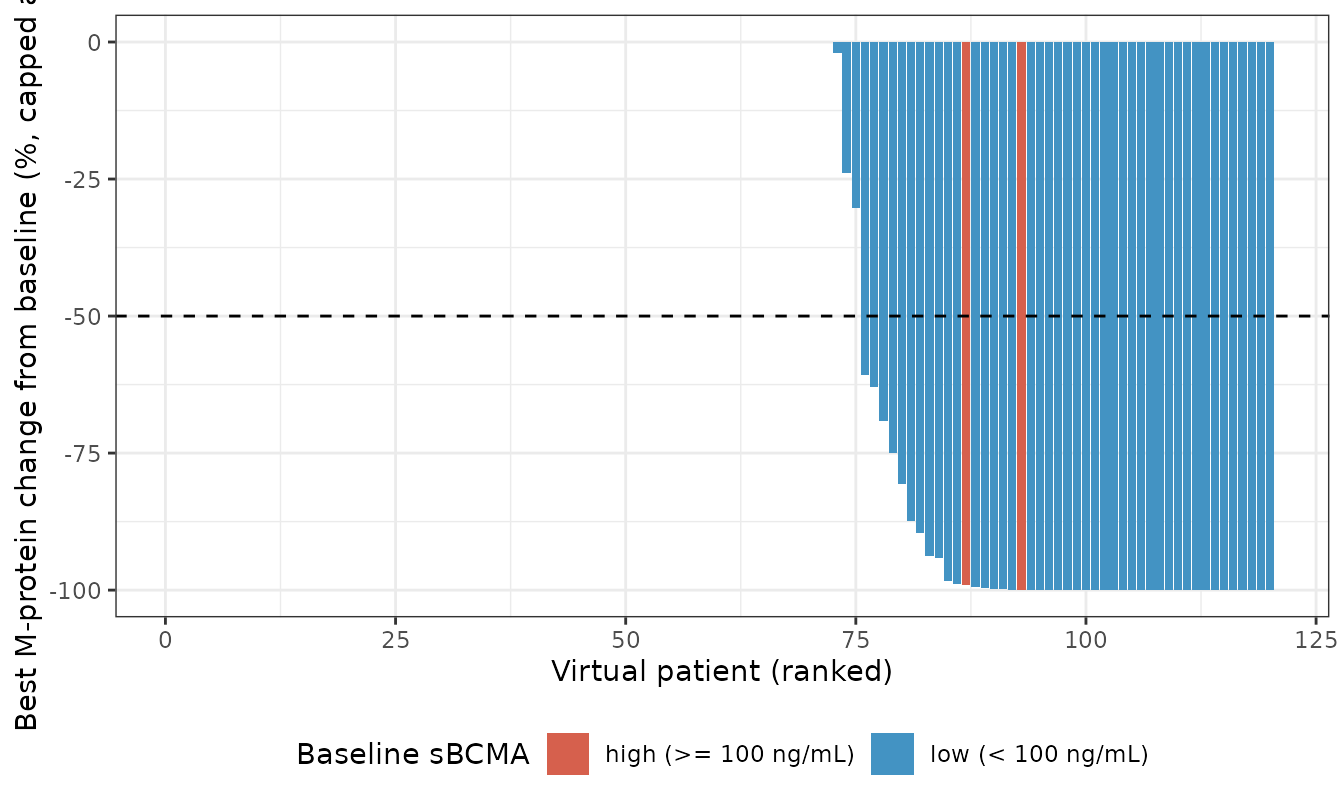
Best M-protein change from baseline for each plausible patient at 76 mg QW, ranked. Compare the waterfall of Figure 2d.
Dose reduction after response (Figure 5)
The paper’s most counter-intuitive result is that stepping down from weekly to Q2W (and then Q4W) dosing in responders improves maintenance of response, because lowering drug exposure frees CD3 receptors from non-productive BsAb-CD3 dimers and lets more trimers form.
horizon <- 18 * CYCLE_H
switch_q2w <- 6 * CYCLE_H     # start of cycle 7
switch_q4w <- 12 * CYCLE_H    # start of cycle 13

sched_qw <- c(prime_time, qw_times(336, horizon))
sched_q2w <- c(prime_time, qw_times(336, switch_q2w - 168),
               seq(switch_q2w, horizon, by = 336))
sched_q4w <- c(prime_time, qw_times(336, switch_q2w - 168),
               seq(switch_q2w, switch_q4w - 336, by = 336),
               seq(switch_q4w, horizon, by = 672))

obs_grid <- seq(0, horizon, by = 6)
step <- dplyr::bind_rows(
  cbind(regimen = "QW throughout",
        solve_qsp(sched_qw, c(prime_mg, rep(76, length(sched_qw) - 3L)), obs_grid)),
  cbind(regimen = "QW -> Q2W at C7",
        solve_qsp(sched_q2w, c(prime_mg, rep(76, length(sched_q2w) - 3L)), obs_grid)),
  cbind(regimen = "QW -> Q2W at C7 -> Q4W at C13",
        solve_qsp(sched_q4w, c(prime_mg, rep(76, length(sched_q4w) - 3L)), obs_grid))
)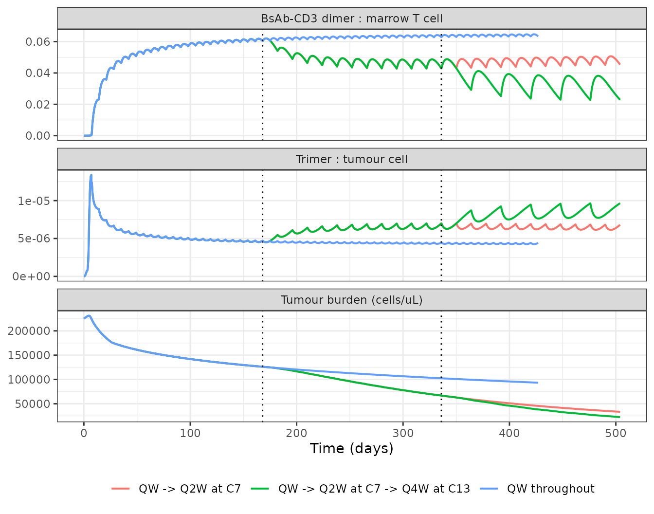
Effect of dose-frequency reduction. Replicates Figure 5a (tumour burden), Figure 5c (trimer per tumour cell) and Supplementary Figure 5a (BsAb-CD3 dimer per T cell).
| Regimen | Mean trimer : tumour cell | Mean BsAb-CD3 dimer : T cell | Tumour burden at C13 | Tumour burden at C18 |
|---|---|---|---|---|
| QW -> Q2W at C7 | 6.3e-06 | 0.0484 | 66810 | 33440 |
| QW -> Q2W at C7 -> Q4W at C13 | 7.2e-06 | 0.0417 | 66810 | 22530 |
| QW throughout | 4.4e-06 | 0.0633 | 102500 | 93360 |
Switching to Q2W at cycle 7 raises the mean trimer-per-tumour-cell ratio over cycles 7-18 from 4.4e-06 to 6.3e-06 while lowering the BsAb-CD3 dimer per marrow T cell from 0.063 to 0.048 – the exact mechanism the paper proposes, and reproduced here from the equations alone. Tumour burden at cycle 13 is 35% lower under the step-down regimen.
Claims checked
| Claim | Source | Checked by |
|---|---|---|
| T cells hold their baseline exactly in the untreated system | Suppl Sects 1.1.1, 1.2.1, Eqs 6 and 28 | Max relative drift < 1e-6 in both compartments (asserted) |
| Untreated cytokine relaxes to the basal balance beta_prod/kdeg_cyt | Suppl Table 3, Eq 7 | Agreement to < 1e-3 pg/mL (asserted) |
| Untreated doubling time equals log(2)/kg0 at low burden | Suppl Table 3, Eq 24 | Fitted slope within 1% (asserted) |
| The logistic term measurably slows growth at higher burden | Suppl Eq 24 | Reference-patient doubling time > 1.05x the low-burden value (asserted) |
| Single-dose Tmax consistent with the label | ELREXFIO USPI 12.3 | Simulated Tmax within 1 day of the 7-day median (asserted) |
| Terminal half-life consistent with the label | ELREXFIO USPI 12.3 | NCA t1/2 within 2-fold of 22 days (asserted) |
| Steady-state clearance consistent with the label | ELREXFIO USPI 12.3 | Dose/AUCtau at week 24 within 2-fold of 0.324 L/day (asserted) |
| Simulated concentrations never go negative | numerical hygiene | all(Cc >= 0) for single-dose and steady-state runs (asserted) |
| Cytokine peaks attenuate over repeated doses | Suppl Fig 8, Eq 37 | Peaks monotone non-increasing; basal by dose 6 (asserted) |
| The Eq 37 reset is what causes the attenuation | Suppl Eq 37 | Peaks higher with the reset suppressed (asserted) |
| Trimer formation is non-monotone in dose (bell shape) | Fig 4a, Suppl Fig 10 | Interior maximum for the reference patient (asserted) |
| More than one dose-response curve shape arises | Suppl Fig 10a | >= 2 distinct shapes across T-cell phenotypes (asserted) |
| Response is lost above ~100 ng/mL baseline sBCMA | Fig 2a, Methods | Highest responding level >= 100 and lowest failing level <= 200 ng/mL (asserted) |
| sBCMA acts through trimer suppression | Fig 3a, Discussion | Mean trimer falls > 10-fold across the range (asserted) |
| ~70% of the virtual population has low baseline sBCMA | Results, Fig 3a | Share between 60% and 80% (asserted) |
| BRR is higher in the low-sBCMA stratum | Fig 3a | brr_low > brr_high (asserted) |
| QW -> Q2W raises the trimer:tumour-cell ratio | Fig 5c | Mean ratio higher after switch (asserted) |
| QW -> Q2W lowers the BsAb-CD3 dimer:T-cell ratio | Suppl Fig 5a | Mean ratio lower after switch (asserted) |
| Dose reduction gives greater tumour shrinkage | Fig 5a | Lower burden at C13 and C18 (asserted) |
Every row marked “asserted” is backed by a stopifnot()
in the chunk that computes it, so this vignette fails to render if any
of them regresses.
Two published results are not reproduced here, and should not be read into the tables above: the absolute biochemical response rates (which depend on the genetic-algorithm virtual-patient selection, see above), and the simulated progressive-disease rates of Figure 5b (which require the same selection step plus the paper’s persistent-responder enrolment logic).
Assumptions and deviations
Values not published, chosen here
- Baseline state defaults. Supplementary Table 2 publishes sampling ranges, not point estimates, for baseline sBCMA, T cells, myeloma burden, M-protein and FLC – the paper has no “typical” patient. The shipped defaults are the geometric midpoint of each published range (Figure 2b confirms all are strongly right-skewed), except myeloma burden, whose range starts at zero and therefore uses the arithmetic midpoint, and M-protein, whose geometric midpoint is taken over 5-70 g/L using the IMWG measurability floor of 0.5 g/dL that the paper itself cites. None of these is a published estimate.
-
Numerical stabiliser
eps_kill. Supplementary Section 1.2.2 introducesepsilonas “a small value introduced for numerical stability” in the trimer:myeloma-cell ratio and gives no value. It is a solver guard, not a calibrated quantity; the default 1e-6 cells/uL is twelve orders of magnitude below the smallest baseline burden in the sampling range. - Log-uniform baseline sampling in the virtual population. The paper states the nine parameters of Supplementary Table 1 were sampled uniformly, and this vignette follows that exactly. For the baseline states it says only that distributions were “fitted to Pfizer baseline clinical data”; those distributions are not published. Figure 2b shows them strongly right-skewed, and drawing them log-uniformly over the Table 2 ranges reproduces the paper’s stated ~70%/30% low/high sBCMA split (a linear-uniform draw gives ~12%/88%).
Published values that conflict with each other
- Myeloma-cell transit time. Supplementary Table 1 gives a default of 27 h with a sampling range of 24-30 h; Supplementary Table 3 gives 24 h. Every other Table 1 default agrees exactly with Table 3, and Table 1’s 27 h is the midpoint of its own range. The model uses Table 3’s 24 h as the authoritative full-parameter-table value; the virtual population samples 24-30 h per Table 1.
-
Baseline circulating cytokine. Supplementary Table
2 initialises the central cytokine state at 2.857 pg/mL, but the model’s
own basal balance is
beta_prod / kdeg_cyt= 2.00 pg/mL. Both are transcribed as published; an untreated simulation relaxes from one to the other within a few hours. - M-protein units in Figure 2b. Figure 2b labels the M-protein axis “(g/dL)” over a 0-65 range, but Supplementary Table 2 gives M-protein in g/L with a 0-70 range, and the paper elsewhere quotes the IMWG measurability threshold as 0.5 g/dL (= 5 g/L). 65 g/dL of M-protein is not physically possible, so the figure axis label is in error and the model uses g/L.
- Mixed units in Supplementary Table 3. Clearance is reported in mL/h (13.9583) while inter-compartmental clearance on the adjacent row is in L/h (0.008416). Each row is transcribed on the units printed for that row; the resulting CL of 0.335 L/day cross-checks against the independent label value of 0.324 L/day, which confirms the reading.
Equations transcribed with a documented correction or caveat
-
Resistance onset (Supplementary Section 1.2.2). As
printed,
km_kill = km * (1 + alpha_resis * (1 - exp(-beta_resis * (t - tau_resis))))diverges to large negative half-maximal kill values beforet = tau_resis(exp(+0.1 * 600)is of order 1e26), which contradicts the stated meaning oftau_resisas “the time it takes for the resistance to occur”. The elapsed time is floored at zero, so resistance is absent untiltau_resisand then rises toalpha_resis. This is the only equation changed from its printed form. -
Mass balance of the marrow BsAb-sBCMA dimer.
Supplementary Eq 17 places the factor
V_BM / V_con the loss ofcomplex_bonemarrowas well as on its gain in the central compartment (Eq 4); the free-drug pair (Eqs 1 and 13) carries that factor on the gain term only. The printed dimer pair is therefore not mass-conserving. It is transcribed exactly as printed. -
Steady-state marrow baselines. The supplement
asserts twice that the system is at steady state at
t = 0, but Supplementary Table 2 lists the marrow T-cell and marrow sBCMA states as independently sampled over the same ranges as their central counterparts. Their ODEs (Eqs 14 and 28) are stationary att = 0only when the marrow value equals the central value times the transport ratio, so the model derives the two marrow baselines from the steady-state relations. Initialising them independently would leave the untreated system with an immediate transient in both, breaking the paper’s own premise. With the derived values, T cells hold their baseline exactly and indefinitely (their dynamics are independent of tumour burden), while sBCMA is stationary only att = 0and thereafter rises with the growing untreated tumour, as Supplementary Eq 14 requires. -
Peripheral and subcutaneous ODEs. Supplementary
Note 1 writes out the central-compartment equation (Eq 1) but not
d/dt(Ab_sc)ord/dt(Ab_p). Both follow uniquely from Eq 1’s own terms and the tabulatedka,F,Q,Vc,Vp:k12 = Q/Vcandk21 = Q/Vpreproduce Eq 1’sk21 * (Vp/Vc) * [Ab_p]term exactly. -
Dose-counter reset delivered from the event table.
Supplementary Eq 37 is a discrete reassignment of
caucat each dose, which no rxode2 ODE can express. It is emitted as anevid = 6multiply record byPoels_2025_elranatamab_qsp_events(). Computing the multiplier there rather than inmodel()keeps it independent of rxode2’s internal ordering of same-time dose records;Poels_2025_elranatamab_qsp_cauc_multiplier()exposes the formula and is unit-tested against the printed equation.
Tabulated but unused
Supplementary Table 3 lists a cytokine-release priming factor
K = 2.83 and a dose counter N
= 1 sourced to Chen et al. (2019), but neither symbol appears
in any printed equation of Supplementary Note 1. They are not carried in
ini(), because an unreferenced parameter would be a
convention violation, and are recorded here instead.
Encoding choices
-
Imax_TCis listed as “Estimated” in Supplementary Table 3 with a value of exactly 1 – the upper bound of a maximum-inhibition fraction. It is encoded asfixed(1)rather than log-transformed, so a refit cannot push it above 1. - Parameters the paper reports as estimated or calibrated are
log-transformed so a refit stays positive; parameters fixed from
nonclinical data, literature or the upstream preliminary popPK are
carried inside
fixed(). - The paper reports no residual-error model and no between-subject
random effects, so
propSdisfixed(0)and the model declares noetaterms.