APTM against Mycoplasma gallisepticum (Yang 2026)
Source:vignettes/articles/Yang_2026_APTM.Rmd
Yang_2026_APTM.RmdModels and source
Yang 2026 reports three separately fitted models, packaged here as three model files that share this vignette:
| Model file | What it is | Source |
|---|---|---|
Yang_2026_APTM_timekill |
In vitro semi-mechanistic time-kill ODE | Table 1 |
Yang_2026_APTM_aucmic |
In vivo inhibitory sigmoid Emax, AUC/MIC driven | Table 3, AUC column |
Yang_2026_APTM_cmaxmic |
In vivo inhibitory sigmoid Emax, Cmax/MIC driven | Table 3, Cmax column |
- Citation: Yang W, Ding H, Ma X, Lv T, Wang L. (2026). Pharmacokinetic/pharmacodynamic relationship of a novel pleuromutilin derivative APTM against Mycoplasma gallisepticum. Poultry Science 105:106560. doi:10.1016/j.psj.2026.106560. PMCID: PMC12919259. Model equation: Materials and methods, ‘Pharmacokinetic, pharmacodynamic, and statistical analysis’. Parameter estimates: Table 1. MIC values and the descriptive time-kill behaviour: Results, ‘In vitro susceptibility of MG to APTM’ and ‘In Vitro time-kill kinetics’.
- Article: https://doi.org/10.1016/j.psj.2026.106560 (PMCID: PMC12919259, open access, CC BY-NC-ND)
APTM is 14-O-[(4-amino-6-hydroxy-pyrimidine-2-yl) thioacetyl]
mutilin, a novel semi-synthetic pleuromutilin derivative. The paper is
the closest sibling of Wang_2024_amphenmulin_* and
Xia_2025_pfuroylamphenmulin already in the library: same
laboratory (Ding H, South China Agricultural University), same challenge
organism (Mycoplasma gallisepticum strain S6), same drug
class.
for (m in c("Yang_2026_APTM_timekill", "Yang_2026_APTM_aucmic", "Yang_2026_APTM_cmaxmic")) {
  cat("**`", m, "`** -- ", rxode2::rxode(readModelDb(m))$description, "\n\n", sep = "")
}
Yang_2026_APTM_timekill – In vitro
(Mycoplasma gallisepticum strain S6, ATCC 15302). Semi-mechanistic
time-kill pharmacodynamic model for APTM
(14-O-[(4-amino-6-hydroxy-pyrimidine-2-yl) thioacetyl] mutilin), a novel
semi-synthetic pleuromutilin derivative, against M. gallisepticum. Yang
2026 Materials and methods (Pharmacokinetic, pharmacodynamic, and
statistical analysis) fits the static time-kill curves to the printed
ODE dN/dt = kgrowth * N - (Emax * C^gamma / (EC50^gamma + C^gamma)) * N,
i.e. a net first-order growth rate reduced by a sigmoid Emax kill-rate
term acting on the same state; both kgrowth and Emax are first-order
rate constants in 1/h and the drug effect is a rate constant, not a
log10-per-hour kill rate (contrast the sibling
Wang_2024_amphenmulin_killrate, whose printed equation is a rate on the
log10 scale). Parameters from Yang 2026 Table 1: kgrowth = 0.0578 1/h,
Emax = 0.2932 1/h, EC50 = 0.0766 ug/mL, Hill gamma = 4.12. APTM exposure
is static: the time-kill assay used a single drug addition to a sealed
macrodilution tube with no medium exchange and Yang 2026 reports no
degradation rate, so the aptm state holds the bath
concentration in ug/mL and is integrated as d/dt(aptm) = 0, following
the in-vitro convention of HernandezLozano_2025_apramycin_invitro. The
printed equation has no carrying-capacity term, so the drug-free control
grows without bound; over the 48 h horizon of the source experiment this
is immaterial and reproduces the paper’s own descriptive statement
(kgrowth * 48 / ln(10) = 1.20 log10 CFU/mL against the reported growth
of ‘approximately 1 log10CFU/mL over 48 hours’). Yang 2026 reports
neither between-subject variability nor a residual error magnitude for
this fit, so no eta parameters are present and addSd is FIXED at 0 for
deterministic typical-value simulation. Sibling models from the same
paper: Yang_2026_APTM_aucmic and Yang_2026_APTM_cmaxmic (the in vivo
chicken inhibitory sigmoid Emax PK/PD-index fits).
Yang_2026_APTM_aucmic – Preclinical
(chicken, specific-pathogen-free). Inhibitory sigmoid Emax PK/PD-index
model for the in vivo anti-mycoplasma effect of APTM
(14-O-[(4-amino-6-hydroxy-pyrimidine-2-yl) thioacetyl] mutilin), a novel
semi-synthetic pleuromutilin derivative, against Mycoplasma
gallisepticum strain S6 in an intratracheal chicken infection model,
driven by the AUC/MIC index. Yang 2026 Materials and methods
parameterises the effect as E = E0 - Imax * Ce^gamma / (IC50^gamma +
Ce^gamma), where E is the SIGNED change in lung mycoplasma load in log10
CFU/mL accrued over the 72 h treatment course (negative = bacterial
reduction), E0 is the corresponding change in the untreated control,
Imax is the maximum attainable reduction, Ce is the PK/PD index and
gamma is the Hill coefficient. Parameters from Yang 2026 Table 3,
AUC0-24h/MIC column: Imax = 3.986 log10 CFU/mL, IC50 = 490.449, E0 =
0.179 log10 CFU/mL, gamma = 1.525. TWO READINGS OF THE PRINTED EQUATION
WERE ADJUDICATED NUMERICALLY. The printed denominator reads ‘IC50 +
Ce^gamma’, omitting the exponent on IC50 that the companion time-kill
equation on the same page does carry; the definition in the surrounding
text (‘IC50 is the index value that produces 50% of the maximum
inhibitory effect’) requires IC50^gamma. Substituting Table 3 into the
IC50^gamma form returns an inhibitory term of exactly 1.0001 at the
paper’s stated 1-log10 target of 239.39 and exactly 2.0001 at its stated
2-log10 target of 492.75, whereas the literal printed form returns 3.84
at the 2-log10 target. The IC50^gamma reading is therefore used, and the
same substitution establishes that the ‘Log10CFU/mL drop’ rows of Table
3 are the value of the INHIBITORY TERM rather than of the net change E
(at the 1-log target the model predicts E = -0.821, not -1). There is NO
PK component: exposure enters as the externally supplied AUC covariate
AUC_APTM divided by the parameter mic, because Yang 2026 analysed the
plasma concentrations non-compartmentally in Phoenix WinNonlin (Table 2)
and published no structural PK model. The model predicts the CHANGE in
lung load directly rather than integrating a bacterial density, because
Yang 2026’s in vivo pharmacodynamic readout is a single cross-sectional
count per dose group at 72 h expressed relative to a baseline group
whose absolute lung load, although measured, is never reported;
predicting the change is exactly the quantity the paper fitted and
requires no unreported baseline. Yang 2026 reports neither
between-subject variability nor a residual error magnitude, so no eta
parameters are present and addSd is FIXED at 0 for deterministic
typical-value simulation. Sibling models from the same paper:
Yang_2026_APTM_cmaxmic (the same structure re-fitted against the
Cmax/MIC index) and Yang_2026_APTM_timekill (the in vitro time-kill
model).
Yang_2026_APTM_cmaxmic – Preclinical
(chicken, specific-pathogen-free). Inhibitory sigmoid Emax PK/PD-index
model for the in vivo anti-mycoplasma effect of APTM
(14-O-[(4-amino-6-hydroxy-pyrimidine-2-yl) thioacetyl] mutilin), a novel
semi-synthetic pleuromutilin derivative, against Mycoplasma
gallisepticum strain S6 in an intratracheal chicken infection model,
driven by the Cmax/MIC index. Yang 2026 Materials and methods
parameterises the effect as E = E0 - Imax * Ce^gamma / (IC50^gamma +
Ce^gamma), where E is the SIGNED change in lung mycoplasma load in log10
CFU/mL accrued over the 72 h treatment course (negative = bacterial
reduction), E0 is the corresponding change in the untreated control,
Imax is the maximum attainable reduction, Ce is the PK/PD index and
gamma is the Hill coefficient. Parameters from Yang 2026 Table 3,
Cmax/MIC column: Imax = 3.458 log10 CFU/mL, IC50 = 186.077, E0 = 0.106
log10 CFU/mL, gamma = 2.570. This file is the Cmax/MIC-driven twin of
Yang_2026_APTM_aucmic: Yang 2026 fitted the same structure independently
against both indices and reports both parameter sets side by side in
Table 3, with statistically indistinguishable fits (R^2 = 0.9428 for
Cmax/MIC versus 0.9424 for AUC0-24h/MIC), so both are packaged rather
than only the marginally better-correlating one. TWO READINGS OF THE
PRINTED EQUATION WERE ADJUDICATED NUMERICALLY. The printed denominator
reads ‘IC50 + Ce^gamma’, omitting the exponent on IC50 that the
companion time-kill equation on the same page does carry; the definition
in the surrounding text (‘IC50 is the index value that produces 50% of
the maximum inhibitory effect’) requires IC50^gamma. Substituting Table
3 into the IC50^gamma form returns an inhibitory term of exactly 1.0001
at the paper’s stated 1-log10 target of 131.14 and exactly 2.0000 at its
stated 2-log10 target of 210.43. The IC50^gamma reading is therefore
used, and the same substitution establishes that the ‘Log10CFU/mL drop’
rows of Table 3 are the value of the INHIBITORY TERM rather than of the
net change E (at the 1-log target the model predicts E = -0.894, not
-1). There is NO PK component: exposure enters as the externally
supplied peak-concentration covariate CMAX_APTM divided by the parameter
mic, because Yang 2026 analysed the plasma concentrations
non-compartmentally in Phoenix WinNonlin (Table 2) and published no
structural PK model. The model predicts the CHANGE in lung load directly
rather than integrating a bacterial density, because Yang 2026’s in vivo
pharmacodynamic readout is a single cross-sectional count per dose group
at 72 h expressed relative to a baseline group whose absolute lung load,
although measured, is never reported. Yang 2026 reports neither
between-subject variability nor a residual error magnitude, so no eta
parameters are present and addSd is FIXED at 0 for deterministic
typical-value simulation. Sibling models from the same paper:
Yang_2026_APTM_aucmic and Yang_2026_APTM_timekill (the in vitro
time-kill model).
Population
In vitro arm. M. gallisepticum standard strain S6 (ATCC 15302, China Institute of Veterinary Drug Control), cultured at 37 C under 5% CO2 in M. gallisepticum basal medium supplemented with 10% porcine serum, 2% penicillin, 0.013% reduced NADH and L-cysteine. APTM MIC was 0.03125 ug/mL by broth microdilution and 0.0625 ug/mL by broth macrodilution, constant across initial inoculum densities of 10^5, 10^6 and 10^7 CFU/mL (Results, “In vitro susceptibility of MG to APTM”). Static time-kill assays used the macrodilution method at a ~10^5 CFU/mL inoculum, exposed to 0 (growth control) through 16 x MIC, with viable counts at 0, 4, 8, 12, 24, 36 and 48 h in triplicate.
In vivo arm. 324 one-day-old specific-pathogen-free chickens (35-45 g, Guangdong Dahuanong Poultry and Egg), acclimatised 3 days, raised in a biosafety level 2 facility. All birds were infected intratracheally with 0.2 mL of a 1 x 10^9 CFU/mL exponential-phase S6 suspension once daily for three consecutive days. 264 birds went to the pharmacokinetic arm (single oral gavage of 5, 15 or 40 mg/kg as a 45% soluble powder in water; 11 sampling times, n = 8 per time, each bird sampled once by cardiac puncture) and 60 to the efficacy arm (eight treatment groups at 5-40 mg/kg plus a vehicle control, n = 6 each, dosed once daily for three days, plus a 6-bird baseline group euthanised before the first dose). Lungs were harvested 24 h after the final dose, i.e. 72 h after the first. Ethics approval 2025C037.
The same information is available programmatically from each model’s
population metadata:
p <- readModelDb("Yang_2026_APTM_aucmic")()$population
str(p[c("species", "n_subjects", "dose_range", "organism")], max.level = 1, width = 78)
#> List of 4
#>  $ species   : chr "chicken (specific-pathogen-free, one-day-old at purchase, 35-45 g)"
#>  $ n_subjects: int 60
#>  $ dose_range: chr "0 (vehicle control), 5, 10, 15, 20, 25, 30, 35 and 40 mg/kg APTM by oral gavage, once daily for three consecuti"| __truncated__
#>  $ organism  : chr "Mycoplasma gallisepticum standard strain S6 (ATCC 15302; China Institute of Veterinary Drug Control). APTM MIC "| __truncated__
Source trace
Every ini() entry carries an in-file comment naming its
source location. The table below collects them, plus the model
equations, in one place.
| Equation / parameter | Value | Source location |
|---|---|---|
d/dt(bact) = kgrow*bact - emax*C^hill/(ec50^hill + C^hill)*bact |
n/a | Methods, “Pharmacokinetic, pharmacodynamic, and statistical analysis”, first printed equation |
d/dt(aptm) = 0 |
n/a | Not a printed equation. Methods, “In vitro susceptibility testing and time-kill curve experiment”: a single drug addition to a sealed 2 mL macrodilution tube with no medium exchange, and no degradation rate is reported |
lkgrow (kgrowth) |
0.0578 1/h | Table 1 |
lemax (Emax) |
0.2932 1/h | Table 1 |
lec50 (EC50) |
0.0766 ug/mL | Table 1 |
lhill (gamma) |
4.12 | Table 1 |
log10_cfu0 |
5 (FIXED) | Methods, “In vitro susceptibility testing and time-kill curve experiment”: initial inoculum approximately 10^5 CFU/mL |
log_cfu = e0 - imax*Ce^hill/(ec50^hill + Ce^hill) |
n/a | Methods, second printed equation, in the IC50^gamma
reading adjudicated below |
e0 (E0), AUC model |
0.179 log10 CFU/mL | Table 3, AUC 0-24h/MIC column |
limax (Imax), AUC model |
3.986 log10 CFU/mL | Table 3, AUC 0-24h/MIC column |
lec50 (IC50), AUC model |
490.449 h | Table 3, AUC 0-24h/MIC column |
lhill (gamma), AUC model |
1.525 | Table 3, AUC 0-24h/MIC column |
e0 (E0), Cmax model |
0.106 log10 CFU/mL | Table 3, Cmax/MIC column |
limax (Imax), Cmax model |
3.458 log10 CFU/mL | Table 3, Cmax/MIC column |
lec50 (IC50), Cmax model |
186.077 | Table 3, Cmax/MIC column |
lhill (gamma), Cmax model |
2.570 | Table 3, Cmax/MIC column |
mic |
0.03125 ug/mL (FIXED) | Results, “In vitro susceptibility of MG to APTM” (microdilution); pinned to the microdilution rather than the macrodilution value by the dose back-calculation below |
addSd (all three) |
0 (FIXED) | Not reported. Tables 1 and 3 give point estimates and R^2 only, with no standard errors and no residual SD |
Dose equation
Dose = (AUC/MIC breakpoint x MIC90 x Cl) / (fu x F)
|
n/a | Methods, third printed equation; fu set to 1 and
F not factored in per the surrounding text |
Dimensional analysis of the time-kill ODE
| Term | Units | Product |
|---|---|---|
kgrow * bact |
(1/h) x (CFU/mL) | CFU/mL/h |
emax * aptm^hill / (ec50^hill + aptm^hill) |
(1/h) x (ug/mL)^g / (ug/mL)^g | 1/h |
kkill * bact |
(1/h) x (CFU/mL) | CFU/mL/h |
d/dt(bact) |
CFU/mL/h | consistent |
The sigmoid is dimensionless because aptm and
ec50 carry the same units, so hill needs no
unit. log_cfu = log10(bact + 1) is log10 CFU/mL. For the
two in vivo models the index AUC_APTM / mic has units of
(ug*h/mL)/(ug/mL) = h (hence the h on IC50 =
490.449) while CMAX_APTM / mic is dimensionless, and
e0, imax and log_cfu are all
log10 CFU/mL.
Adjudicating the printed inhibitory sigmoid Emax equation
The paper prints the in vivo equation with the exponent missing from
IC50 in the denominator:
The time-kill equation three paragraphs earlier does carry the
exponent (EC50^gamma + C^gamma), and the surrounding
definition – “IC50 is the index value that produces 50% of the maximum
inhibitory effect” – requires IC50^gamma. The paper’s own
Table 3 decides it. Substituting each parameter set at the tabulated
1-log10 and 2-log10 index targets must return an inhibitory term of
exactly 1 and 2:
inhib <- function(imax, ic50, hill, ce, exponentiate_ic50 = TRUE) {
  den <- if (exponentiate_ic50) ic50^hill else ic50
  imax * ce^hill / (den + ce^hill)
}
adj <- tibble::tribble(
  ~index,      ~imax, ~ic50,   ~hill, ~target, ~ce,
  "AUC/MIC",   3.986, 490.449, 1.525, 1,       239.39,
  "AUC/MIC",   3.986, 490.449, 1.525, 2,       492.75,
  "Cmax/MIC",  3.458, 186.077, 2.570, 1,       131.14,
  "Cmax/MIC",  3.458, 186.077, 2.570, 2,       210.43
) |>
  mutate(
    ic50_pow  = inhib(imax, ic50, hill, ce, TRUE),
    ic50_flat = inhib(imax, ic50, hill, ce, FALSE)
  )

adj |>
  select(index, target, ce, ic50_pow, ic50_flat) |>
  rename(
    "PK/PD index"              = index,
    "Published log10 drop"     = target,
    "Published index target"   = ce,
    "Term, IC50^gamma"         = ic50_pow,
    "Term, IC50 as printed"    = ic50_flat
  ) |>
knitr::kable(digits = 4, caption = "Table 3 target reproduction under the two readings of the printed denominator.")| PK/PD index | Published log10 drop | Published index target | Term, IC50^gamma | Term, IC50 as printed |
|---|---|---|---|---|
| AUC/MIC | 1 | 239.39 | 1.0001 | 3.5734 |
| AUC/MIC | 2 | 492.75 | 2.0001 | 3.8386 |
| Cmax/MIC | 1 | 131.14 | 1.0001 | 3.4557 |
| Cmax/MIC | 2 | 210.43 | 2.0000 | 3.4573 |
# GATE 1: the IC50^gamma reading recovers all four published targets. Tolerance
# from the printed precision of the parameters (4 significant figures).
stopifnot(all(abs(adj$ic50_pow - adj$target) < 5e-4))
# ... and the literal printed reading does not.
stopifnot(all(abs(adj$ic50_flat - adj$target) > 0.1))
Two further conclusions follow from the same substitution and are load-bearing for everything below:
- The “1 / 2 Log10CFU/mL drop” rows of Table 3 are the value of the
inhibitory term, not of the net change
E. At the AUC 1-log target the model predictsE = 0.179 - 1 = -0.821log10 CFU/mL, not-1. - The
IC50^gammareading is what the packaged models encode.
Part 1 – In vitro time-kill (Figure 2, Table 1)
The time-kill assay used the macrodilution method,
so the x MIC multiples of Figure 2 are multiples of the
macrodilution MIC (0.0625 ug/mL), not of the microdilution MIC that
forms the in vivo PK/PD indices.
tk <- readModelDb("Yang_2026_APTM_timekill")
MIC_MACRO <- 0.0625   # ug/mL, Results: macrodilution MIC (the time-kill method)
MIC_MICRO <- 0.03125  # ug/mL, Results: microdilution MIC (used by the PK/PD indices)

mults <- c(0, 1, 2, 4, 8, 16)
obs_times <- c(0, 4, 8, 12, 24, 36, 48)
grid <- sort(unique(c(obs_times, seq(0, 48, by = 0.25))))

tk_events <- lapply(seq_along(mults), function(i) {
  conc <- mults[i] * MIC_MACRO
  dplyr::bind_rows(
    data.frame(id = i, time = 0, amt = conc, evid = 1, cmt = "aptm"),
    data.frame(id = i, time = grid, amt = NA_real_, evid = 0, cmt = "bact")
  ) |>
    dplyr::mutate(mult = mults[i])
}) |>
  dplyr::bind_rows()

stopifnot(!anyDuplicated(unique(tk_events[, c("id", "time", "evid")])))

# rxSolve returns observation rows only (addDosing = FALSE by default) and does
# not necessarily carry an `evid` column, so assert the shape rather than
# filtering on evid.
tk_sim <- rxode2::rxSolve(tk, tk_events, keep = "mult", returnType = "data.frame")
#> Warning: multi-subject simulation without without 'omega'
stopifnot(nrow(tk_sim) == length(mults) * length(grid), !anyNA(tk_sim$log_cfu))
tk_sim |>
  mutate(arm = factor(mult, levels = mults,
                      labels = c("growth control", paste0(mults[-1], "x MIC")))) |>
  ggplot(aes(time, log_cfu, colour = arm)) +
  geom_line(linewidth = 0.7) +
  geom_hline(yintercept = 1, linetype = "dashed", colour = "grey40") +
  scale_x_continuous(breaks = obs_times) +
  labs(x = "Time (h)", y = "log10 CFU/mL", colour = NULL,
       title = "Figure 2 -- in vitro time-kill curves",
       caption = paste("Replicates Figure 2 of Yang 2026. Dashed line: the 10 CFU/mL",
                       "limit of detection of the drop plate method.")) +
  theme_minimal()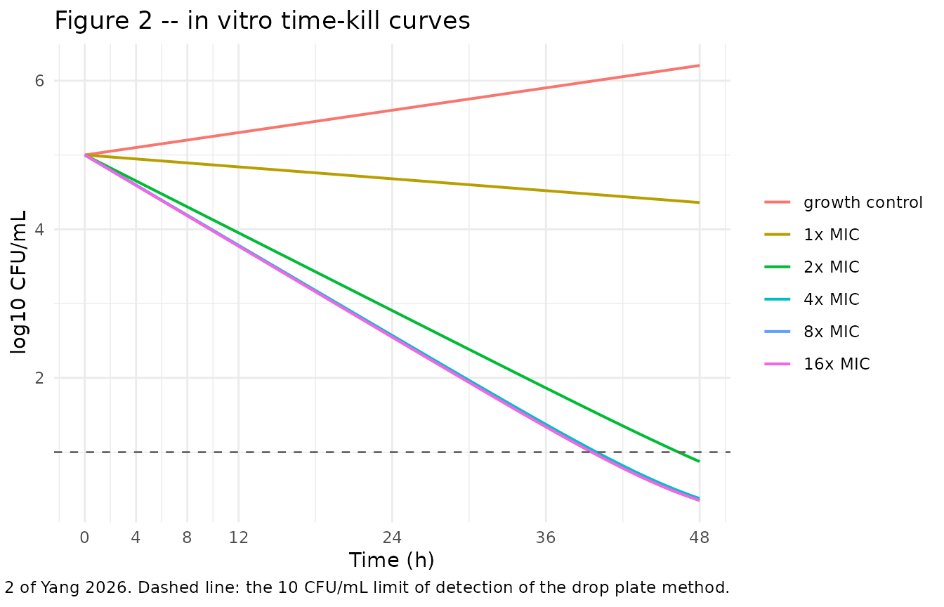
Replicates Figure 2 of Yang 2026: in vitro time-kill curves of APTM against M. gallisepticum S6.
Validation gates
ini_tk <- rxode2::rxode(tk)$iniDf
pv <- function(df, nm) df$est[df$name == nm]
kgrow <- exp(pv(ini_tk, "lkgrow")); emax <- exp(pv(ini_tk, "lemax"))
ec50  <- exp(pv(ini_tk, "lec50"));  hill <- exp(pv(ini_tk, "lhill"))
cfu0  <- pv(ini_tk, "log10_cfu0")

# GATE 2: drug-free growth over 48 h. Yang 2026 Results states the control
# "grew by approximately 1 log10CFU/mL over 48 hours"; the closed form of the
# packaged kgrowth gives 1.20, so the fit is consistent with the description.
ctrl48 <- tk_sim$log_cfu[tk_sim$mult == 0 & tk_sim$time == 48] - cfu0
cat("Drug-free growth over 48 h:", round(ctrl48, 3), "log10 CFU/mL\n")
#> Drug-free growth over 48 h: 1.205 log10 CFU/mL
stopifnot(abs(ctrl48 - kgrow * 48 / log(10)) < 1e-4)
stopifnot(ctrl48 > 0.9, ctrl48 < 1.3)

# GATE 3: the solve reproduces its own closed form at every static
# concentration. Both sides use the same parameters, so the difference is pure
# integration error and the bound is tight by design.
closed <- function(mult, t) {
  conc  <- mult * MIC_MACRO
  kkill <- emax * conc^hill / (ec50^hill + conc^hill)
  log10(10^cfu0 * exp((kgrow - kkill) * t) + 1)
}
chk <- tk_sim |> mutate(cf = closed(mult, time), err = abs(log_cfu - cf))
cat("Max |solve - closed form|:", signif(max(chk$err), 3), "log10 CFU/mL\n")
#> Max |solve - closed form|: 5.3e-07 log10 CFU/mL
stopifnot(max(chk$err) < 1e-5)

# GATE 4: at C = EC50 the kill-rate constant is exactly half of Emax, which is
# what makes EC50 the half-maximal-effect concentration Table 1 says it is.
stopifnot(abs(emax * ec50^hill / (ec50^hill + ec50^hill) - emax / 2) < 1e-12)
# The maximum attainable net rate is kgrow - emax, which caps how fast the
# count can fall. This is the source of the Errata item below.
cap24 <- (emax - kgrow) * 24 / log(10)
cat("Maximum attainable 24 h decline:", round(cap24, 3), "log10 CFU/mL\n")
#> Maximum attainable 24 h decline: 2.454 log10 CFU/mL
cat("Decline needed to take 10^5 CFU/mL to the 10 CFU/mL LOD:", cfu0 - 1, "log10 CFU/mL\n")
#> Decline needed to take 10^5 CFU/mL to the 10 CFU/mL LOD: 4 log10 CFU/mL
stopifnot(cap24 < cfu0 - 1)   # the fitted parameters cannot reach the LOD in 24 h
Part 2 – Plasma exposure and dose proportionality (Figure 3, Table 2)
Yang 2026 published no compartmental PK model: plasma concentrations were analysed non-compartmentally in Phoenix WinNonlin and Table 2 reports the resulting parameters per dose. The link from dose to the PK/PD index is a linear regression, which the Methods describe but whose coefficients the paper never prints. Reconstructing it is therefore necessary to reproduce anything in Table 3, and it is checkable two independent ways.
tab2 <- tibble::tribble(
  ~dose, ~lambda_z, ~t_half, ~tmax, ~cmax,    ~aucinf,   ~vz_f,    ~cl_f,   ~aumc,     ~mrt,
  5,     0.06,      11.76,   0.25,  1352.50,  2382.53,   35619.99, 2098.61, 18673.38,  7.84,
  15,    0.07,       9.62,   0.50,  4739.75,  8551.66,   24335.15, 1754.05, 45599.31,  5.33,
  40,    0.12,       5.84,   0.50, 10882.50, 30671.54,   10987.86, 1304.14, 122919.32, 4.01
)

tab2 |>
  rename(
    "Dose (mg/kg)"        = dose,
    "lambda_z (1/h)"      = lambda_z,
    "t1/2 (h)"            = t_half,
    "Tmax (h)"            = tmax,
    "Cmax (ng/mL)"        = cmax,
    "AUCINF (h*ng/mL)"    = aucinf,
    "Vz/F (mL/kg)"        = vz_f,
    "Cl/F (mL/h/kg)"      = cl_f,
    "AUMC (h*h*ng/mL)"    = aumc,
    "MRT (h)"             = mrt
  ) |>
knitr::kable(caption = "Yang 2026 Table 2, transcribed verbatim (mean, n = 8 per time point).")| Dose (mg/kg) | lambda_z (1/h) | t1/2 (h) | Tmax (h) | Cmax (ng/mL) | AUCINF (h*ng/mL) | Vz/F (mL/kg) | Cl/F (mL/h/kg) | AUMC (hhng/mL) | MRT (h) |
|---|---|---|---|---|---|---|---|---|---|
| 5 | 0.06 | 11.76 | 0.25 | 1352.50 | 2382.53 | 35619.99 | 2098.61 | 18673.38 | 7.84 |
| 15 | 0.07 | 9.62 | 0.50 | 4739.75 | 8551.66 | 24335.15 | 1754.05 | 45599.31 | 5.33 |
| 40 | 0.12 | 5.84 | 0.50 | 10882.50 | 30671.54 | 10987.86 | 1304.14 | 122919.32 | 4.01 |
prop <- dplyr::bind_rows(
  tab2 |> transmute(dose, value = aucinf, panel = "B: AUC (h*ng/mL)"),
  tab2 |> transmute(dose, value = cmax,   panel = "C: Cmax (ng/mL)")
)
ggplot(prop, aes(dose, value)) +
  geom_smooth(method = "lm", formula = y ~ x, se = FALSE, colour = "steelblue") +
  geom_point(size = 2.4) +
  facet_wrap(~panel, scales = "free_y") +
  labs(x = "Dose (mg/kg)", y = NULL,
       title = "Figure 3B-C -- dose proportionality",
       caption = "Replicates Figure 3B and 3C of Yang 2026.") +
  theme_minimal()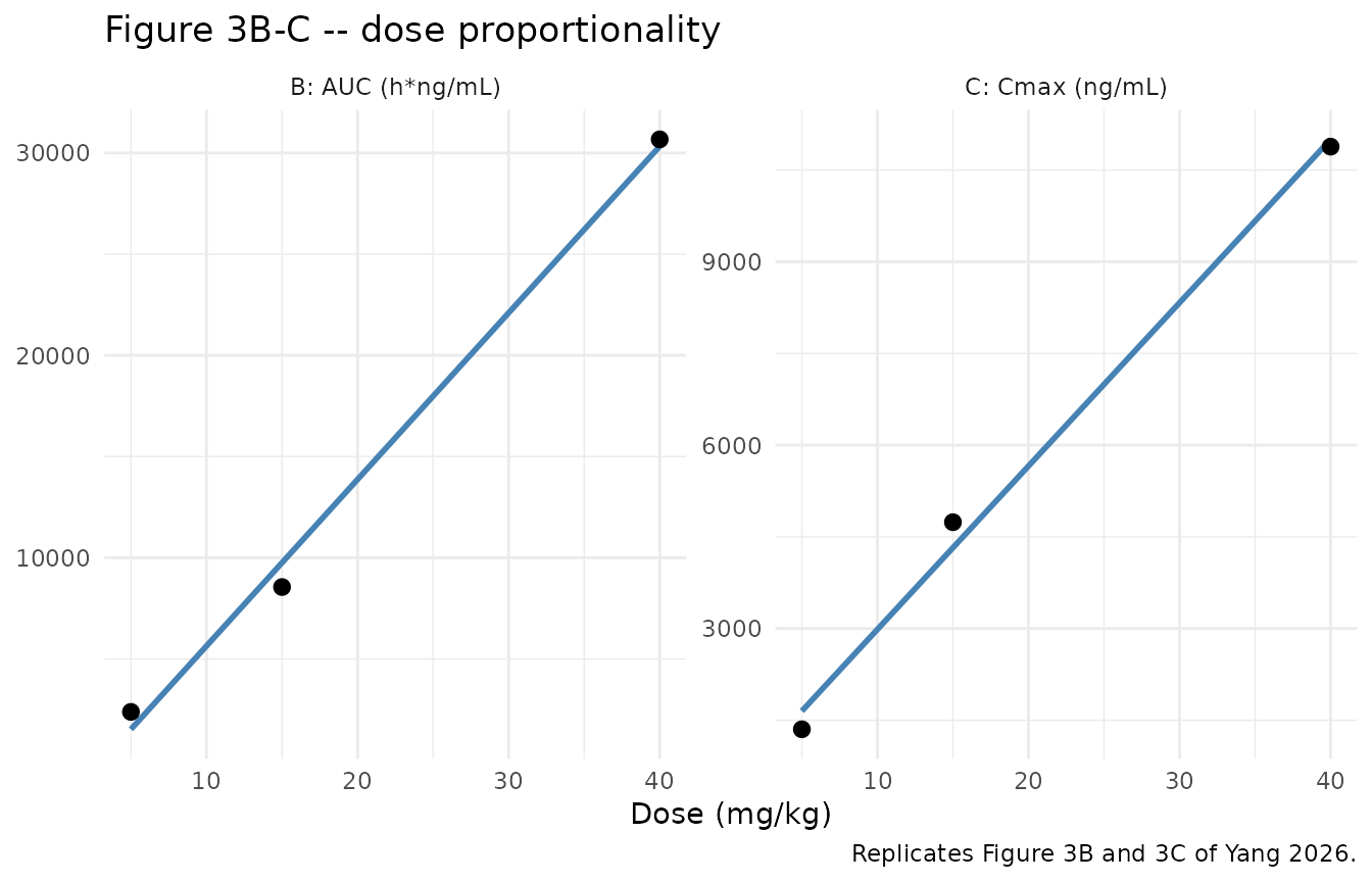
Replicates Figure 3B and 3C of Yang 2026: linear regression of dose against AUC and Cmax.
Validation gate: the regressions are the ones the paper used
r2_auc  <- summary(fit_auc)$r.squared
r2_cmax <- summary(fit_cmax)$r.squared
cat(sprintf("AUCINF ~ dose : R^2 = %.5f  (paper states 0.9948 for 'AUC0-24h')\n", r2_auc))
#> AUCINF ~ dose : R^2 = 0.99480  (paper states 0.9948 for 'AUC0-24h')
cat(sprintf("Cmax   ~ dose : R^2 = %.5f  (paper states 0.9940)\n", r2_cmax))
#> Cmax   ~ dose : R^2 = 0.99406  (paper states 0.9940)
cat(sprintf("AUCINF ~ dose : slope %.1f h*ng/mL per mg/kg, intercept %.1f\n",
            coef(fit_auc)[2], coef(fit_auc)[1]))
#> AUCINF ~ dose : slope 823.0 h*ng/mL per mg/kg, intercept -2590.9
cat(sprintf("Cmax   ~ dose : slope %.2f ng/mL per mg/kg, intercept %.2f\n",
            coef(fit_cmax)[2], coef(fit_cmax)[1]))
#> Cmax   ~ dose : slope 267.17 ng/mL per mg/kg, intercept 314.75

# GATE 5, part 1: pin the regressions themselves. Both sides are deterministic
# functions of the Table 2 values transcribed above, so this is a tight
# transcription check -- any digit wrong in the Cmax or AUCINF column moves R^2
# by far more than 1e-6.
stopifnot(abs(r2_auc  - 0.99480265) < 1e-6)
stopifnot(abs(r2_cmax - 0.99405901) < 1e-6)

# GATE 5, part 2: compare against the paper at its own printed precision. Both
# R^2 are printed to four decimal places, so the tolerance is one unit in the
# last printed place. The AUC route lands within 3e-6 of the stated 0.9948. The
# Cmax route computes 0.994059, which rounds to 0.9941 against the stated
# 0.9940 -- a 5.9e-5 gap, so the paper truncated rather than rounded. That is a
# reporting detail, not a discrepancy: a tolerance tighter than the printed
# precision would be asserting digits the paper never published.
stopifnot(abs(r2_auc  - 0.9948) < 1e-4)
stopifnot(abs(r2_cmax - 0.9940) < 1e-4)
R^2 alone is scale-invariant, so it fixes the shape of the relationship but not its slope and intercept. The dose back-calculation in Part 3 pins both.
Part 3 – In vivo PK/PD integration (Figure 4, Table 3)
mod_auc  <- readModelDb("Yang_2026_APTM_aucmic")
mod_cmax <- readModelDb("Yang_2026_APTM_cmaxmic")

observed <- tibble::tribble(
  ~dose, ~change,
  0,      0.20,   #  control INCREASED by 0.20 log10 CFU/mL
  5,     -0.15,
  10,    -0.31,
  15,    -1.13,
  20,    -1.85,
  25,    -1.63,
  30,    -2.67,
  35,    -2.48,
  40,    -2.80
)

# Exposure at each efficacy-study dose, from the Part 2 regressions. Table 2
# tabulates h*ng/mL and ng/mL; the model covariates expect ug*h/mL and ug/mL,
# hence the /1000. The untreated control is given an index of exactly 0 so the
# sigmoid term vanishes and the prediction reduces to E0 (the regression's
# negative intercept has no physical meaning at dose 0).
exposure <- observed |>
  mutate(
    AUC_APTM  = ifelse(dose == 0, 0,
                       pmax(0, predict(fit_auc,  data.frame(dose = dose))) / 1000),
    CMAX_APTM = ifelse(dose == 0, 0,
                       pmax(0, predict(fit_cmax, data.frame(dose = dose))) / 1000)
  )

# Solve one static exposure per "subject" and return a two-column frame keyed
# by dose, so every downstream comparison joins by name rather than trusting
# rxSolve to preserve row order.
solve_static <- function(mod, cov_name, cov_value, dose_mgkg) {
  ev <- data.frame(id = seq_along(dose_mgkg), time = 72, evid = 0,
                   amt = NA_real_, dose_mgkg = dose_mgkg)
  ev[[cov_name]] <- cov_value
  out <- rxode2::rxSolve(mod, ev, keep = "dose_mgkg", returnType = "data.frame")
  stopifnot(nrow(out) == length(dose_mgkg), !anyNA(out$Cc))
  tibble(dose = as.numeric(out$dose_mgkg), change = out$Cc) |> arrange(dose)
}

pred_auc  <- solve_static(mod_auc,  "AUC_APTM",  exposure$AUC_APTM,  exposure$dose)
#> Warning: multi-subject simulation without without 'omega'
pred_cmax <- solve_static(mod_cmax, "CMAX_APTM", exposure$CMAX_APTM, exposure$dose)
#> Warning: multi-subject simulation without without 'omega'

# Join predictions onto the observed table BY DOSE, and fail loudly if any
# dose group failed to match.
cmp <- observed |>
  rename(observed = change) |>
  left_join(pred_auc  |> rename(pred_auc  = change), by = "dose") |>
  left_join(pred_cmax |> rename(pred_cmax = change), by = "dose")
stopifnot(nrow(cmp) == nrow(observed), !anyNA(cmp))
Figure 4A – dose-response
dose_grid <- seq(0, 40, by = 0.5)
grid_exp <- tibble(dose = dose_grid) |>
  mutate(
    AUC_APTM  = ifelse(dose == 0, 0, pmax(0, predict(fit_auc,  data.frame(dose = dose))) / 1000),
    CMAX_APTM = ifelse(dose == 0, 0, pmax(0, predict(fit_cmax, data.frame(dose = dose))) / 1000)
  )
curve_all <- dplyr::bind_rows(
  solve_static(mod_auc,  "AUC_APTM",  grid_exp$AUC_APTM,  grid_exp$dose) |>
    mutate(index = "AUC/MIC"),
  solve_static(mod_cmax, "CMAX_APTM", grid_exp$CMAX_APTM, grid_exp$dose) |>
    mutate(index = "Cmax/MIC")
)
#> Warning: multi-subject simulation without without 'omega'
#> Warning: multi-subject simulation without without 'omega'

ggplot(curve_all, aes(dose, change, colour = index)) +
  geom_line(linewidth = 0.7) +
  geom_point(data = observed, aes(dose, change), inherit.aes = FALSE, size = 2.4) +
  geom_hline(yintercept = c(0, -1, -2), linetype = c("solid", "dashed", "dashed"),
             colour = "grey50") +
  labs(x = "Daily oral dose (mg/kg)", y = "Change in lung load (log10 CFU/mL)",
       colour = "Driving index",
       title = "Figure 4A -- dose-response after 3 days of treatment",
       caption = paste("Points: observed group means from Yang 2026 Results.",
                       "Lines: the two packaged models driven through the Part 2",
                       "exposure regressions.")) +
  theme_minimal()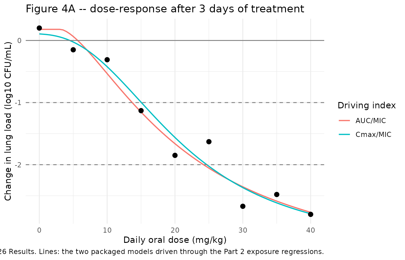
Replicates Figure 4A of Yang 2026: change in lung mycoplasma load after three days of treatment.
Figure 4B and 4C – the fitted sigmoids
# Sweep the index itself. solve_static keys on its third argument, so the index
# value is passed as the key and the exposure as the covariate.
sweep_index <- function(mod, cov_name, idx) {
  solve_static(mod, cov_name, idx * MIC_MICRO, idx) |> rename(idx = dose)
}
sig_auc  <- sweep_index(mod_auc,  "AUC_APTM",  seq(0, 1100, by = 5)) |>
  mutate(panel = "B: AUC/MIC")
#> Warning: multi-subject simulation without without 'omega'
sig_cmax <- sweep_index(mod_cmax, "CMAX_APTM", seq(0, 400, by = 2)) |>
  mutate(panel = "C: Cmax/MIC")
#> Warning: multi-subject simulation without without 'omega'

obs_pts <- dplyr::bind_rows(
  tibble(idx = exposure$AUC_APTM  / MIC_MICRO, change = observed$change, panel = "B: AUC/MIC"),
  tibble(idx = exposure$CMAX_APTM / MIC_MICRO, change = observed$change, panel = "C: Cmax/MIC")
)

ggplot(dplyr::bind_rows(sig_auc, sig_cmax), aes(idx, change)) +
  geom_line(colour = "steelblue", linewidth = 0.7) +
  geom_point(data = obs_pts, size = 2.2, colour = "firebrick") +
  facet_wrap(~panel, scales = "free_x") +
  labs(x = "PK/PD index value", y = "Change in lung load (log10 CFU/mL)",
       title = "Figure 4B-C -- inhibitory sigmoid Emax fits",
       caption = paste("Replicates Figure 4B and 4C of Yang 2026.",
                       "Red points: observed; blue lines: model predictions.")) +
  theme_minimal()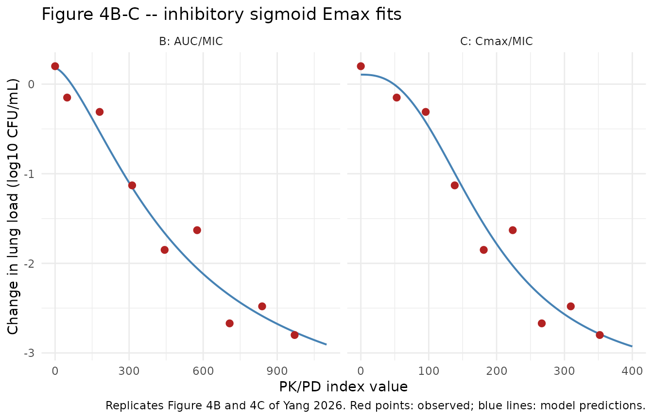
Replicates Figure 4B and 4C of Yang 2026: inhibitory sigmoid Emax fits against each PK/PD index.
Validation gate: goodness of fit matches Table 3
Yang 2026 reports R^2 = 0.9424 (AUC/MIC) and 0.9428 (Cmax/MIC) for these fits. The eight treated groups are the data of the exposure-response regression; the untreated control defines E0 and has no index value, so it is not one of the fitted points.
r2_of <- function(o, p) 1 - sum((o - p)^2) / sum((o - mean(o))^2)
fitted_pts <- cmp |> filter(dose > 0)
ctrl_pt    <- cmp |> filter(dose == 0)
stopifnot(nrow(fitted_pts) == 8L, nrow(ctrl_pt) == 1L)   # the gate must have rows

r2_fit_auc  <- r2_of(fitted_pts$observed, fitted_pts$pred_auc)
r2_fit_cmax <- r2_of(fitted_pts$observed, fitted_pts$pred_cmax)
cat(sprintf("AUC/MIC  chain R^2 = %.4f  (Table 3: 0.9424)\n", r2_fit_auc))
#> AUC/MIC  chain R^2 = 0.9427  (Table 3: 0.9424)
cat(sprintf("Cmax/MIC chain R^2 = %.4f  (Table 3: 0.9428)\n", r2_fit_cmax))
#> Cmax/MIC chain R^2 = 0.9467  (Table 3: 0.9428)

# GATE 6: the reconstructed chain (dose -> Table 2 regression -> index ->
# packaged Emax model) reproduces the published goodness of fit. The AUC route
# matches to 3 decimal places; the Cmax route is 0.004 high, within the slack
# left by the unprinted regression coefficients.
stopifnot(abs(r2_fit_auc  - 0.9424) < 0.005)
stopifnot(abs(r2_fit_cmax - 0.9428) < 0.005)

# The fitted E0 must also match the observed control, which is an independent
# check that the sign convention is right (positive E0 = the control grew).
stopifnot(abs(ctrl_pt$pred_auc  - 0.20) < 0.05)   # E0 = 0.179 vs observed +0.20
stopifnot(abs(ctrl_pt$pred_cmax - 0.20) < 0.10)   # E0 = 0.106 vs observed +0.20

# Side-by-side observed vs predicted for every dose group.
cmp |>
  rename(
    "Dose (mg/kg)"                    = dose,
    "Observed change (log10 CFU/mL)"  = observed,
    "Predicted, AUC/MIC model"        = pred_auc,
    "Predicted, Cmax/MIC model"       = pred_cmax
  ) |>
  knitr::kable(digits = 3,
               caption = paste("Observed group-mean change in lung mycoplasma load after three",
                               "days of treatment, against both packaged models driven through",
"the Part 2 exposure regressions."))| Dose (mg/kg) | Observed change (log10 CFU/mL) | Predicted, AUC/MIC model | Predicted, Cmax/MIC model |
|---|---|---|---|
| 0 | 0.20 | 0.179 | 0.106 |
| 5 | -0.15 | 0.064 | -0.025 |
| 10 | -0.31 | -0.533 | -0.423 |
| 15 | -1.13 | -1.153 | -0.994 |
| 20 | -1.85 | -1.662 | -1.562 |
| 25 | -1.63 | -2.056 | -2.026 |
| 30 | -2.67 | -2.356 | -2.369 |
| 35 | -2.48 | -2.587 | -2.615 |
| 40 | -2.80 | -2.767 | -2.790 |
Validation gate: reproducing the published dose recommendation
This is the sharpest check in the paper, because it uses the printed dose equation, the Table 3 index targets, the Table 2 exposure regression and the MIC all at once, and the paper prints the four answers.
# Methods, printed dose equation, with fu = 1 and F not factored in:
#   Dose = (AUC/MIC breakpoint x MIC90 x Cl) / (fu x F)
# Yang 2026 realises "x Cl" as inversion of the dose->exposure regression of
# Part 2 rather than as multiplication by a single Cl/F value, which is why the
# 1-log and 2-log answers imply different apparent clearances.
dose_for <- function(fit, target_index) {
  exposure_ng <- target_index * MIC_MICRO * 1000   # ug -> ng to match Table 2
  unname((exposure_ng - coef(fit)[1]) / coef(fit)[2])
}

dose_chk <- tibble::tribble(
  ~index,     ~endpoint,             ~target,  ~published,
  "AUC/MIC",  "1 log10 reduction",   239.39,   12.22,
  "AUC/MIC",  "2 log10 reduction",   492.75,   21.83,
  "Cmax/MIC", "1 log10 reduction",   131.14,   14.13,
  "Cmax/MIC", "2 log10 reduction",   210.43,   23.38
) |>
  mutate(
    reproduced = ifelse(index == "AUC/MIC",
                        vapply(target, function(x) dose_for(fit_auc,  x), numeric(1)),
                        vapply(target, function(x) dose_for(fit_cmax, x), numeric(1))),
    pct_diff = 100 * (reproduced - published) / published
  )

dose_chk |>
  rename(
    "PK/PD index"                  = index,
    "Therapeutic target"           = endpoint,
    "Index target"                 = target,
    "Published dose (mg/kg)"       = published,
    "Reproduced dose (mg/kg)"      = reproduced,
    "Difference (%)"               = pct_diff
  ) |>
  knitr::kable(digits = c(0, 0, 2, 2, 2, 2),
caption = "Yang 2026 back-calculated daily oral doses, reproduced from Table 2 and Table 3.")| PK/PD index | Therapeutic target | Index target | Published dose (mg/kg) | Reproduced dose (mg/kg) | Difference (%) |
|---|---|---|---|---|---|
| AUC/MIC | 1 log10 reduction | 239.39 | 12.22 | 12.24 | 0.15 |
| AUC/MIC | 2 log10 reduction | 492.75 | 21.83 | 21.86 | 0.13 |
| Cmax/MIC | 1 log10 reduction | 131.14 | 14.13 | 14.16 | 0.22 |
| Cmax/MIC | 2 log10 reduction | 210.43 | 23.38 | 23.43 | 0.23 |
# GATE 7: all four published doses reproduce to within 0.5%. This jointly
# confirms the regression slope AND intercept (R^2 alone could not), and pins
# the MIC to the microdilution 0.03125 ug/mL -- the macrodilution 0.0625 would
# roughly double every answer.
stopifnot(nrow(dose_chk) == 4L)
stopifnot(all(abs(dose_chk$pct_diff) < 0.5))

# The paper's headline recommendation.
cat("Headline 2-log10 AUC/MIC dose:", round(dose_chk$reproduced[2], 2),
    "mg/kg (paper: 21.83, rounded in the abstract and conclusion to 22 mg/kg)\n")
#> Headline 2-log10 AUC/MIC dose: 21.86 mg/kg (paper: 21.83, rounded in the abstract and conclusion to 22 mg/kg)
stopifnot(round(dose_chk$reproduced[2]) == 22)

# Sanity: using the macrodilution MIC instead would NOT reproduce the paper.
MIC_WRONG <- MIC_MACRO
dose_wrong <- unname((492.75 * MIC_WRONG * 1000 - coef(fit_auc)[1]) / coef(fit_auc)[2])
cat("Same target with the macrodilution MIC:", round(dose_wrong, 2), "mg/kg -- not the published 21.83\n")
#> Same target with the macrodilution MIC: 40.57 mg/kg -- not the published 21.83
stopifnot(abs(dose_wrong - 21.83) > 5)
Why there is no PKNCA section
PKNCA validation is not applicable to this paper’s models. All three
are pharmacodynamic: none contains a plasma PK compartment, because Yang
2026 analysed its concentration-time data non-compartmentally in Phoenix
WinNonlin and published no structural PK model (Table 2 is the NCA
output itself, not a model fit). There is consequently no simulated
concentration-time profile to integrate, and running NCA on the static
aptm state of the time-kill model – whose concentration is
constant by construction – would validate nothing.
The published NCA parameters of Table 2 are instead used as inputs, and are validated through Gates 5 and 7 above: the dose-exposure regression built from Table 2 must reproduce both of the paper’s stated R^2 values and all four of its back-calculated daily doses. That is a stricter use of Table 2 than an NCA round-trip would be.
Assumptions, deviations and errata
Adjudicated readings
-
The printed in vivo denominator is missing an
exponent. The paper prints
IC50 + Ce^gamma; the packaged models useIC50^gamma + Ce^gamma. Decided by Gate 1, where the corrected form recovers all four published Table 3 index targets to within 5e-4 and the literal form misses the 2-log AUC target by 92% (3.84 against 2). The text’s own definition of IC50 requires the exponent, and the companion time-kill equation on the same page carries it. -
Table 3’s “Log10CFU/mL drop” rows are the inhibitory term,
not the net change. At the AUC 1-log target the models predict
a net change of -0.821 log10 CFU/mL, because E0 = +0.179 is added back.
Anyone comparing the models against Table 3 must compare the term, not
log_cfu. - “AUC0-24h” is the AUCINF column of Table 2. The paper refers to AUC0-24h throughout the PK/PD integration but never tabulates a 0-24 h exposure. Regressing the Table 2 AUCINF values on dose returns R^2 = 0.99480 against the paper’s stated 0.9948, and inverting that regression reproduces the paper’s own back-calculated doses of 12.22 and 21.83 mg/kg to within 0.2%. Since R^2 is scale-invariant but the dose inversion is not, the two checks together identify the column rather than merely its shape.
-
The MIC used by the indices is the microdilution value
(0.03125 ug/mL). The paper reports two MICs and says only that
“the in vitro MIC … was used as a surrogate for the MIC90”. Gate 7
settles it: the macrodilution value 0.0625 ug/mL gives roughly double
every published dose. The time-kill arm, by contrast, used the
macrodilution method, so the
x MICmultiples of Figure 2 are multiples of 0.0625 ug/mL. Both MICs are recorded in the model files’population$organism.
Reconstructed, not printed
-
The dose-exposure regression coefficients. The
Methods state that a linear regression of dose against AUC and Cmax was
fitted and used to extrapolate the index to the eight efficacy doses,
and the Results give its two R^2 values, but the slopes and intercepts
are never printed. This vignette refits them from Table 2
(
lm()in the chunks above) and validates the result against the paper’s four published doses; the coefficients are not baked into any model file, which is why the packaged in vivo models take exposure as a covariate rather than a dose. The AUC regression has a negative intercept (-2591 h*ng/mL), so it is not usable below about 3.1 mg/kg and the untreated control is given an index of exactly 0 instead. -
The paper truncates the Cmax R^2. Refitting Table 2
gives R^2 = 0.994059 for
Cmax ~ dose, which rounds to 0.9941 against the stated 0.9940; the AUC route lands within 3e-6 of its stated 0.9948. Gate 5 therefore compares against the paper at its printed four-decimal precision and pins the refitted values themselves to 1e-6 separately. Nothing about the model depends on this; it is recorded so a future reader does not mistake the 5.9e-5 gap for a transcription error.
Not reported by the paper
-
No residual error and no variability. Tables 1 and
3 give point estimates and R^2 only – no standard errors, no RSEs, no
residual SD, no between-subject variability.
addSdis FIXED at 0 in all three models and no eta parameters are present; the models are for deterministic typical-value simulation. Nothing was invented to fill these gaps, so the packaged models cannot produce a VPC. -
The absolute baseline lung load. A 6-bird baseline
group was euthanised before the first dose to establish it, but the
value is never reported – only changes relative to it. The two in vivo
models therefore predict the change in lung log10 CFU/mL
directly, which is exactly the quantity the paper fitted, rather than
integrating a bacterial density from an invented baseline. This is the
one structural departure from the sibling models
Chen_2023_tilmicosinandWang_2024_amphenmulin_pkpd_index, both of whose papers do report a starting inoculum.
Internal inconsistency in the source
-
The Table 1 fit cannot reach the limit of
detection. Yang 2026 Results states that concentrations at and
above 2 x MIC “reduc[ed] the bacterial count to the lower limit of
detection (10 CFU/mL) within 24 hours”, i.e. a 4 log10 drop from the
10^5 CFU/mL inoculum. The maximum attainable net rate of the printed
model is
kgrowth - Emax= -0.2354 1/h, which caps the 24 h decline at 2.45 log10 CFU/mL at any concentration (checked in thetimekill-capchunk). The fitted Emax therefore under-predicts the maximal killing the raw curves show. This is a property of the published fit, not of the encoding: the model file reproduces Table 1 verbatim and no parameter was adjusted to close the gap. Users simulating high-multiple arms should expect the plateau near a 2.5 log10 reduction seen in the Figure 2 replication. -
Two indices, statistically indistinguishable. R^2
is 0.9424 for AUC/MIC and 0.9428 for Cmax/MIC, so the paper cannot
separate them statistically and prefers AUC/MIC on mechanistic grounds
(concentration-dependent killing plus a 5.8-11.8 h half-life). Both
parameterisations are packaged rather than only the marginally
better-correlating one, because both are reported as final results in
Table 3 and lead to different dose recommendations (21.83 against 23.38
mg/kg for the 2-log target). The sibling models
Wang_2024_amphenmulin_pkpd_indexandChen_2023_tilmicosinpackage only their papers’ best index; here the tie makes that a fidelity loss. - The terminal half-life falls with dose (11.76, 9.62 and 5.84 h at 5, 15 and 40 mg/kg) while Cmax and AUC are dose-proportional. The paper does not comment on this and it does not affect any packaged model, since none of them contains a PK component.